Pre-Processor Tab
The Pre-Processor tab contains the optional pre-processing step.
Load Data
The data must be saved as a .CSV or a .MAT dataset file.
Click the import dataset ![]() icon or use the File menu to navigate to the dataset file. You can select one or
multiple files to load. All files must have the same number of columns and use the same
variable names.
icon or use the File menu to navigate to the dataset file. You can select one or
multiple files to load. All files must have the same number of columns and use the same
variable names.
CSV Dataset File
The .CSV header determines the type of ROM, static or dynamic, that can be generated.
If the first column name is “time,” romAI can be used to generate a static or dynamic ROM. Otherwise, only a static ROM can be generated.
Hence, the first few lines of a .CSV file typically look like the following two examples:


MAT Dataset File
The variables contained in the .mat file determine the type of ROM, static or dynamic, that can be generated.
If a variable called “time” exists, romAI can be used to generate a static or dynamic ROM. Otherwise, only a static ROM can be generated.
The following are two examples of .MAT files.


The variables contained in the .MAT file must be column or row vectors with the same number of elements.
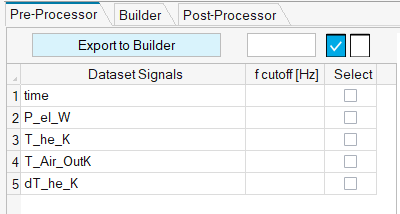
After the dataset file has been loaded, the Signal Table is populated as follows:
Select Data
All data from the loaded dataset file is listed in the Signal Table.
To select a signal, click the check box in the same row of the signal name. To select all
the signals, click the Select All ![]() button. It
plots all the signals on the window.
button. It
plots all the signals on the window.
To deselect all the signals, click the Select None
![]() button
button
Filter Data
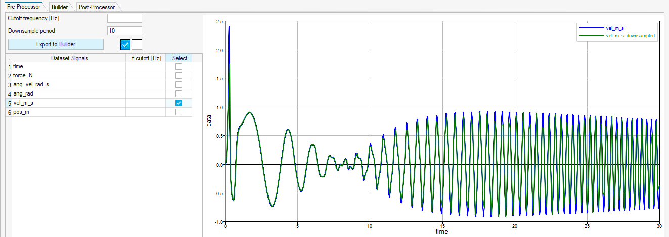
Data can be filtered through a low pass filter with a cutoff frequency.
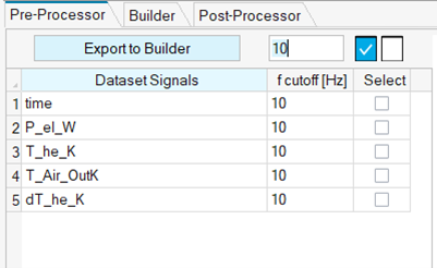
Enter a value in the Cutoff frequency (Hz) field, and then press Enter. This filter will be applied to all the signals in the table.
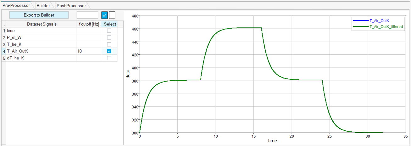
To filter a signal, enter the filter frequency in the f cutoff [Hz] column of that signal. The plot is refreshed automatically and shows the filtered and the baseline data.
To revert the filtering, delete the cutoff frequency value and press Enter. To revert filtering from multiple selected signals, delete the frequency value from filter entry on the top of the table and press Enter.
Downsample Data
Data can be downsampled to speed up the training process.
Plot Data
All data that is listed in the Signal Table can be plotted.
If labels are repeated, they are plotted only once.
To generate plots, select the check box in the same row of the signal name.
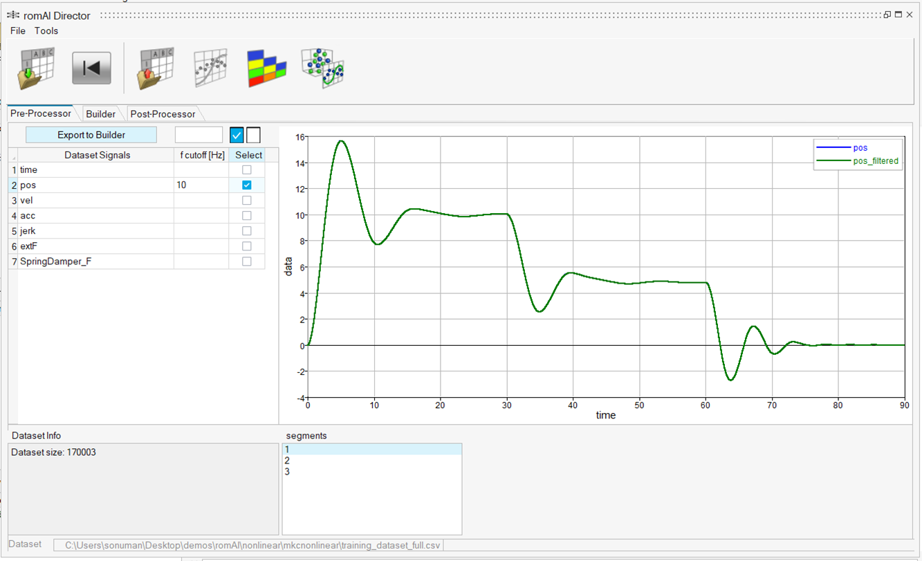
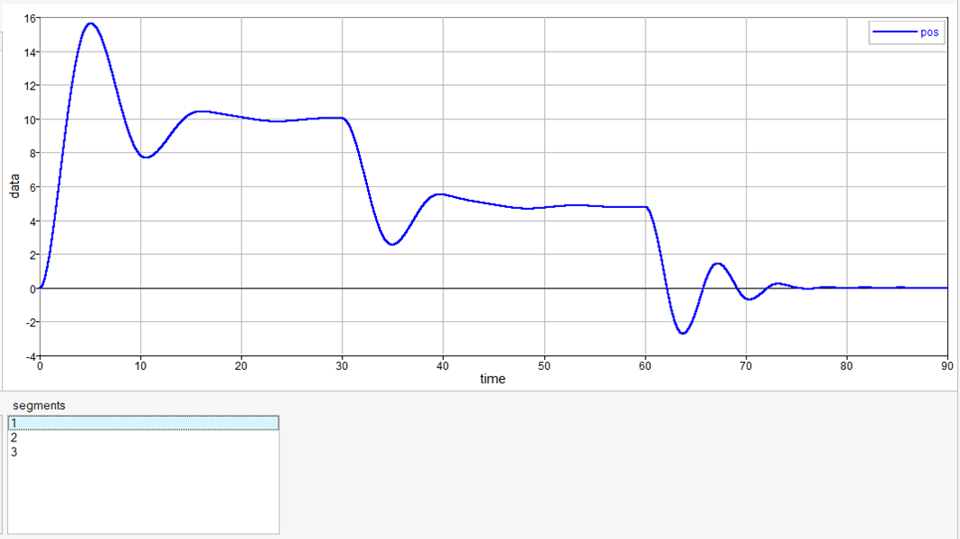
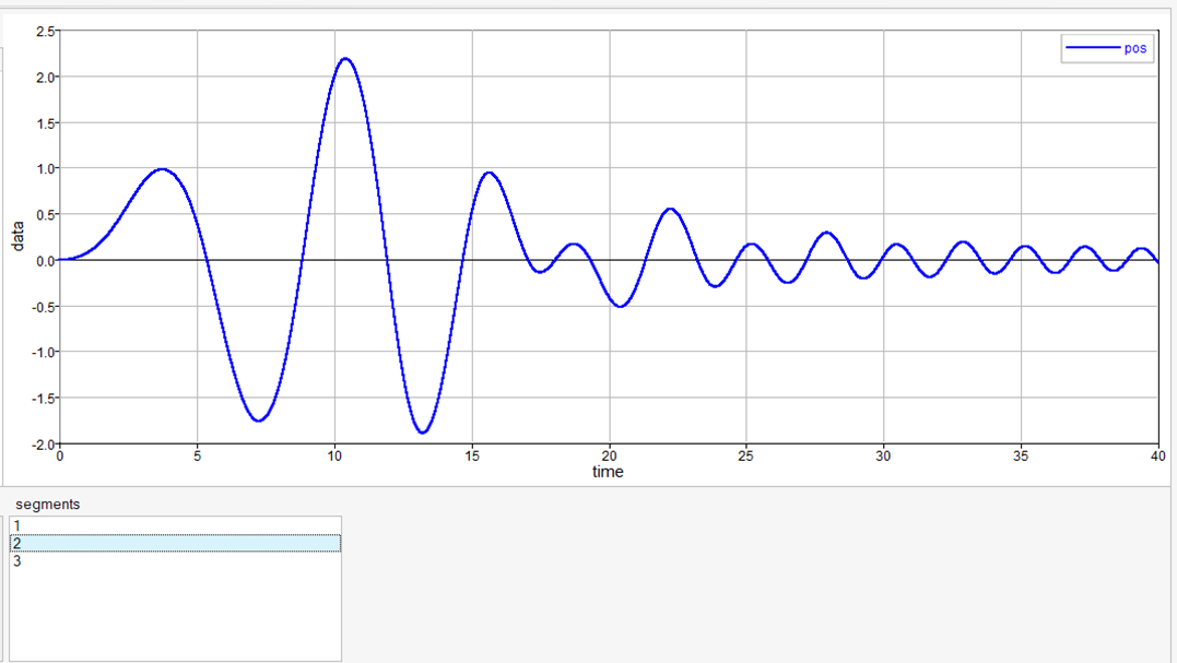
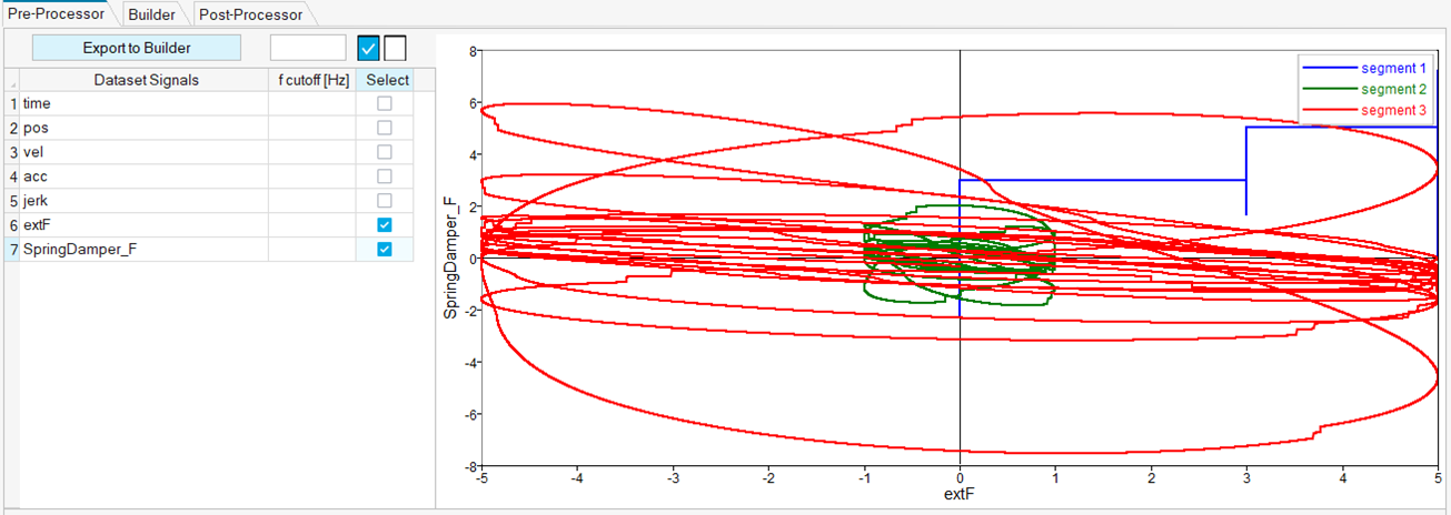
If the time vector is not monotonically increasing, the data is split into segments. The segments can be selected using the segments list box in the panel area.
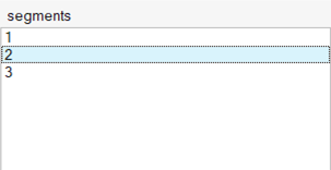
Segments let you view different data segments in the plot.
Heat Map
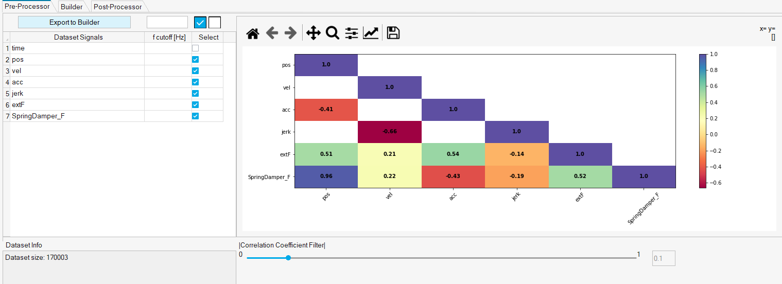
Heat Map can help you choose the input features for the model.
It provides the correlation coefficient values of signals among each other. To plot heat
map, click on the Heat Map
![]() icon in the ribbon. When you click on the Heat
Map icon, the icon is deactivated. The Correlation Coefficient slider
can be used to filter the most correlated features based on the slide value. The slider
value ranges from 0 to 1 where 1 indicates 100 % correlation. The slider value filters
both positive and negatively correlated values.
icon in the ribbon. When you click on the Heat
Map icon, the icon is deactivated. The Correlation Coefficient slider
can be used to filter the most correlated features based on the slide value. The slider
value ranges from 0 to 1 where 1 indicates 100 % correlation. The slider value filters
both positive and negatively correlated values.
To go back to the 2D plot icon, click on the 2D plot
![]() icon
icon
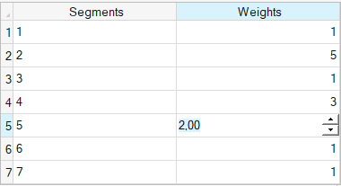
Weights for Segments
Add a weight to a segment.
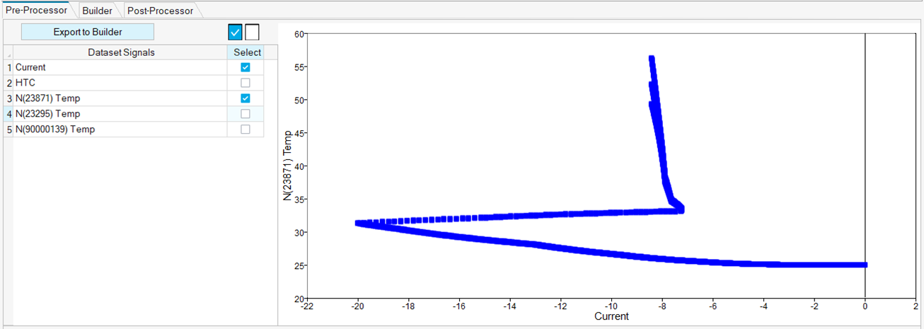
Domain View
Check the variation of a signal with other signals.
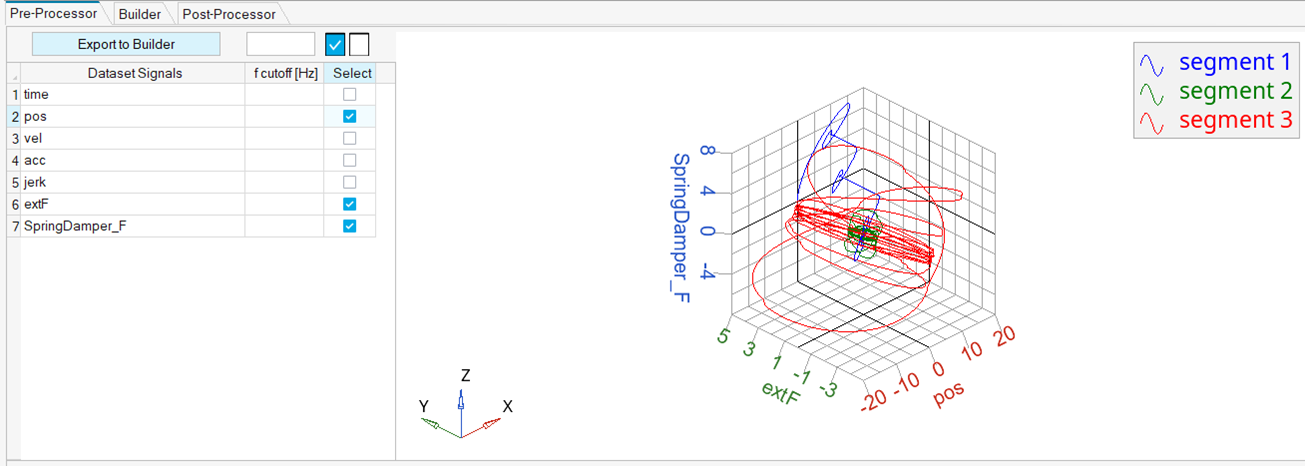
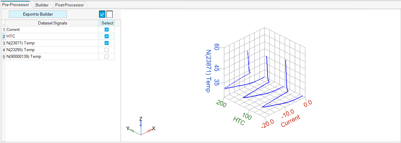
Visualizations
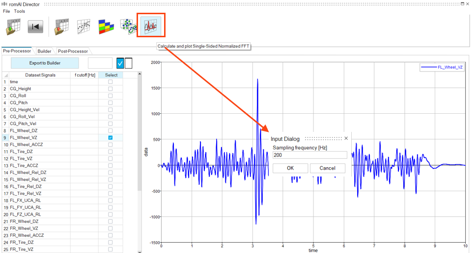
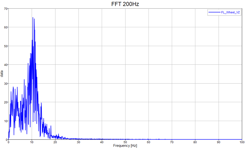
Using the single-sided normalized Fast Fourier Transformation, you move from the time domain visualization of the signal to the frequency domain and thus can explore its frequency content and identify any periodic phenomena.
This can also help to properly select the filter cutoff frequency by making sure you do not cut off frequencies of importance.
Click the Transformation icon and then set the sampling frequency.
Save Data
All selected signals can be saved to an external .CSV file.
icon and specify a file name and directory. The time vector is automatically inserted and saved as the first column of the file.
Export Data
All the selected signals can be exported.
To export to the Builder tab, click the Export to Builder button.
The TrainData File edit box is automatically populated.