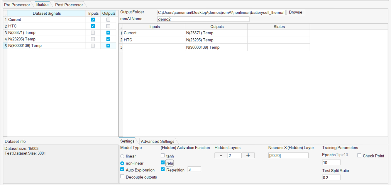
Builder Tab

Import Data

You can import training data in three ways.

Use the Export to Builder button.
Select File > Import Dataset.
Use the Import Dataset

icon to load a dataset file. The selected file name is shown in the File Info panel on the bottom of the dialog box.

Specify the Directory

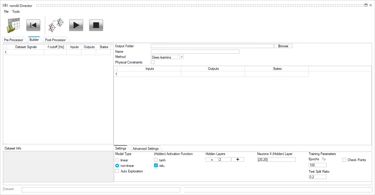
Select the Browse button and navigate to the folder where you want to save the ROM to be trained.

Inside this folder, a subfolder is created. Use the romAI Name text box to enter a name for the subfolder.

Specify the ROM Creation Method

Select a method for the creation of the ROM.

From the Method drop-down list, select Deep learning or SINDy.

Deep learning is the default method and is preferred for most use cases.

When Deep learning is selected, romAI leverages machine learning techniques in combination with classical system theory, whereas SINDy uses sparse regression packages for the system identification.

The Deep learning method can be used to identify both static (state-less) and dynamic systems, whereas SINDy works only with dynamic systems.

SINDy may be used in situations where the approximate equation of the system is required to be identified (white box). SINDy can also be leveraged as a first step before training a model with the romAI method, in order to identify any predominant functions that could be artificially added as inputs of the model.

Define Inputs, Outputs, and States

After you have loaded the data, the Signal Table is automatically populated and you can specify your inputs, outputs, and state variables, as applicable.

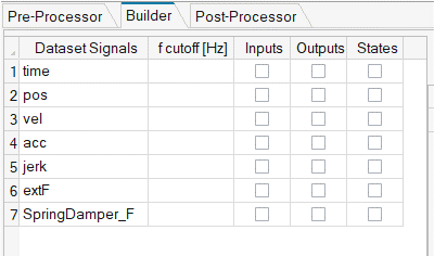
Select the Input, Output, or State using the check box. The Features Table on the right side populate accordingly.

To remove data labels from a desired box, deselect the check box.

You must specify at least one input and one output. State variables are optional. As is common in classical system theory, some, or all, state variables can be outputs as well.

Add and Edit Physical Constraints

Adding physical constraints is an option if state variables exist. If state variables do exist, it is possible for one state variable to be the derivative of another. Since romAI technology is a mix of AI and system modeling techniques, the romAI application can take this into account and produce a better ROM. Hence, it is good practice to specify the derivative variables.

If one or more state variables are specified, the Physical constraints check box is visible.

If you select the check box, a column is added to the Features Table. This column contains the names of the state variables in a drop-down list. Here, you can select the name that specifies which variable is the derivative, if applicable, for each state variable.

For example, given the following set of state variables:

Select the Physical Constraints check box, and the following table appears.

In the State Derivative column, use the drop-down cells to specify the derivatives.

Note: If the Physical Constraints check box is deselected, the physical constraints will not be considered in the ROM.

To clear the derivative column, select an empty cell in a drop-down list. To clear all derivatives, deselect the Physical Constraints check box.

Define the Model Architecture

Deep Learning

The ROM is based on an MLP (multilayer perceptron) structure.

Select a model type:
- linear: The model architecture is defined by default, and no further action is required.
- non linear: Continue to the next step.
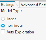
For the (Hidden) Activation Function, select tanh or relu.
Enter the number of hidden layers of the MLP. Click the + and – buttons to increase or decrease the number of hidden layers. You can also type the exact number of layers directly in the text box.
Enter the number of neurons per layer. Type the number in the text box. You can also leverage the OML syntax and type square brackets for matrices, and commas as column separators, as required.

SINDy

Define the SINDy model architecture in the Settings tab.

SINDy uses sparse regression to identify a linear combination of basis functions that most effectively represents the dynamic behavior of the physical system. These basis functions are part of different feature libraries.

Figure 1. Settings Tab when SINDy Method is Selected

Polynomial Library:
- Degree: Relates to the degree (power) of the polynomial features.
- Interaction: If enabled, interaction features are produced (e.g., x₁ * x₃).
- Bias: If enabled, a bias term is included in the feature.
Fourier Library:
- # of frequencies: Relates to the number of frequencies to use on the sine or cosine functions (e.g., sin⁡(x), sin ⁡(2x), … sin⁡ (#_frequenciesx)
- Include sin/cos: If enabled, includes according terms in the feature library.
Library Combination Options:
- In romAI Director, you have the option to use the Polynomial and Fourier feature libraries or a combination of those. You may concatenate (+) or tensor (*) multiple libraries together for more flexibility.

Define Training Parameters

Deep Learning

The training parameters are divided into two parts.

The mandatory parameters are in the Settings tab. Other parameters are in the Advanced Settings tab. Specify the training parameters or keep the provided default values.

The mandatory parameters are outlined in the following table.


Parameter	UI Widget	Description
Test Split Ratio		Enter the ratio of the Dataset for testing.
Epochs		Enter the number of epochs (such as iterations) for the optimization algorithm.
Check Points		Select this option to save the output files at a particular interval of epochs.
Check Points Interval		Enter the epoch interval that should be used to save the intermediate result files.

The epochs parameter provides you with a suggested minimum value that is updated when:

Inputs/Outputs/State variables are removed or added.
Neural net structure (for example, number of layers and/or neurons per layer) is changed.

The suggested minimum value is displayed beside the Epochs edit box.

The default value in other parameters are usually good enough for the model. These parameters are:


Parameter	UI Widget	Description
Regularization Coefficient		Enter the penalty factor of the L2 regularization.
Learning Rate		Enter the Learning Rate.

Another set of training parameters is enabled when you select the Early Stopping check box.


Parameter	UI Widget	Description
Early Stopping		Select this option to stop training when a monitored metric has stopped improving.
Monitor Metric		Select the minimum change in the monitored quantity that qualifies as an improvement: Choose val_loss (validation loss) or val_acc (validation accuracy).
Min Improvement		Enter the minimum change in the monitored quantity that qualifies as an improvement.
Patience		Enter the allowable number of epochs with no improvement that defines when the training stops.
Cross-validation Split Ratio		Enter the ratio of the Training Dataset for cross-validation.

SINDy

Define the training parameters in the Settings tab.

During the fitting process, an optimizer determines the coefficient matrix to minimize the objective function. Currently, only the STLSQ (Sequentially Thresholded Least Squares Algorithm) is available.

Figure 2. Training Parameters in the Settings Tab when SINDy Method is Selected

Threshold: Minimum allowable identified coefficient. Values below this threshold are set to zero.
Regularization Coefficient: Regularization term on the objective function. This helps avoid overfitting and might improve generalization.
Max Iterations: Refers to the maximum iterations the algorithm is allowed to make.

Launch Training

After you have defined the training parameters, move the romAI Director window to the left of the workspace.
Undock the Python window and move it to the right.
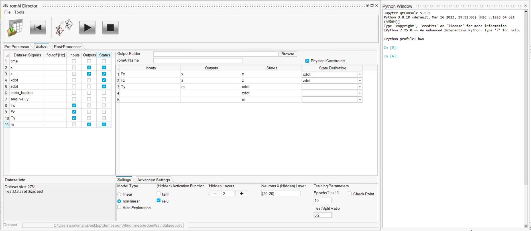
Click the Train icon to launch the training procedure.
After the training begins, you can view the progress in the Python window.

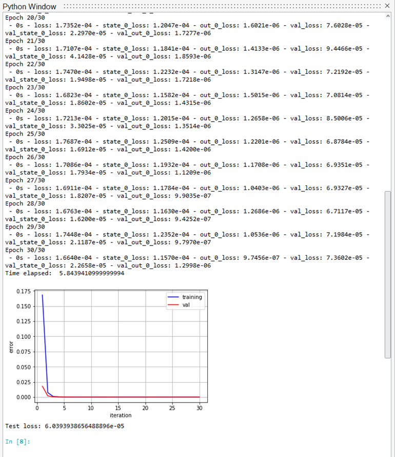
To stop training in between, click the Stop Training icon.
When the training ends, the Post-Processor tab is automatically populated.

Training Output Files

The training produces three files in a subfolder.

The files include:

An .OML file containing the ROM and training parameters information.
A .CSV file containing the training history.
An .H5 file containing the net weights.

Important: Do not add or remove files in the subfolder.

Utilities

Three utilities offer different functions.

Click the Reset button to clear the current Builder session.
Click File > Save Session to save the current Builder session information (dataset, inputs/outputs/states, training parameters, etc.) to an external .OML file.
Click File > Load Session to load a previously-saved Builder session.

Transfer Learning

Use Transfer Learning to train a pre-trained model for more epochs.

Select a training dataset.
Do one of the following:
- Click the Transfer Learning icon, or;
- Select File > Import romAI Model.
The background color of the icon changes , which indicates that the Transfer Learning mode is active. In this mode, only a few options are available. To go back to the normal view, click on the icon again.
Select the Browse button and navigate to folder where you want to save the ROM that is about to be trained. Inside this folder, a subfolder is created.
Enter a name for the subfolder in the Epochs text box.

Note: This field is already populated and contains the epoch value for which the selected model was trained. You can change this value based on your requirements.
Click the Train icon to start the training.

Note: The epoch values are additive. If a model that was trained for X epochs is trained further using transfer learning for another Y epochs, then the resulting model contains history of X+Y epochs.

Decoupled Outputs

In the case of static models, it could be better to divide one single model with multiple outputs into several models with single output.

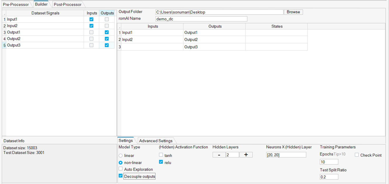
Training a model with single output result in better accuracy as compared to the model where there are multiple outputs. The Decouple outputs option lets you automatically create multiple model with single outputs.

As shown in image above, if the model is trained with Deouple outputs selected, then three models are generated and are stored in a folder named with following syntax: <romAI name>_<output_name>_decoupled<integer>.

The integer in the end is added to avoid overwriting of the model files. The folder name is also shown in the message box which is shown after training.

An Compose OML file is also created along with romAI models with single outputs.

This file contains input, outputs, and folder names and is used by the romAI block to load all the models in one block. In this case user needs to provide the path to the master folder in romAI block.

Optionally, the models with single output can be used as necessary.

Auto Exploration

Auto Exploration allows you to run multiple models with different combinations of activation function, hidden layers, and number of neurons in one click.

Select the Auto Exploration check box.
Select the Activation Function options.
Enter the minimum and maximum number of hidden layers, and the increment step for the hidden layers.
Enter the minimum and maximum number of neurons per layer, and the increment step for the neurons.
Click the Start Training

icon.
All the models generated from Auto Exploration training are put in an auto_<integer> folder. This folder is created inside the output folder. It is done to make the post-processing easy.
There is one more option available in Auto Exploration to repeat the training of the same model. This option can be used to perform a convergence study on the model training. The number of models generated can be specified in the entry box beside the Repetition check box.