Post-Processor Tab
The Post-Processor tab lets you visualize and evaluate the trained ROM.
- Automatic: The Post-Processor tab is automatically updated with results after the training launched in the Builder tab ends.
- Select a previously-trained romAI or a folder that
contain romAI models using the
 icon.
icon.
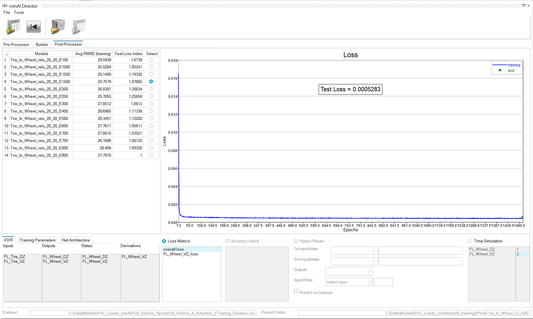
The Parent Folder shows the path of the selected master folder. All the models inside it are listed in the post-table. Next to the model names, the Avg RMSE (training) along with the Test Loss Index columns also get populated in the table.
The Avg RMSE (training) is calculated as the average of all outputs and segments of the root mean square error between the target vs romAI predictions evaluated on the training set. The model with the least RMSE gets automatically selected.
The Test Loss Index column has a minimum value of 1, which represents the model with lowest value of training loss. The other loss values represent the scaling factor of the loss compared to the minimum loss value.
- I/O/S: Inputs, outputs, states (and physical constraints)
- Training Parameters
- Net Architecture parameters
In this phase, you can use the post-processing tools that are provided to evaluate the ROM accuracy.
- Loss Metrics
- Accuracy check
- Hyper PlanesNote: This option is available only where it is applicable. It is not available if the total number of inputs and states are less than two.
- Time Simulation
Check Loss
View the overall training, validation, and test loss.
Select the Loss Metrics radio button.

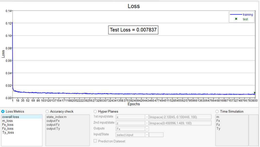
The data also shows the training/validation loss of each single output or higher-order state variable, such as velocity in this case.
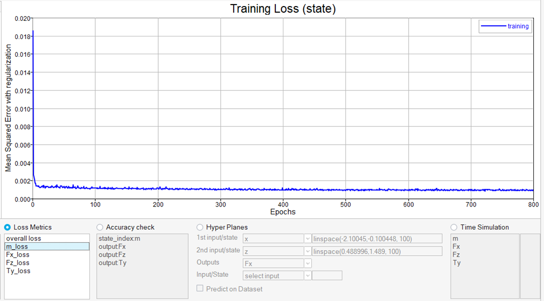
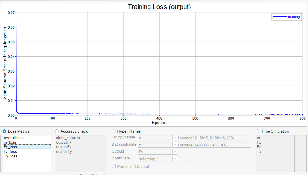
- The lower the training error, the more accurate the ROM.
- If the training and test loss is close to each other, then the training has converged.
- If the training and test losses diverge, then the ROM might be affected by overfitting. In this case, you may want to consider increasing the regularization term.
- The cross-validation ratio is used to monitor the Early Stop criteria. To change the cross-validation ratio, select the Early Stopping check box as shown below.

Check Accuracy
The R2 Accuracy check is applicable only for static models.
In the case of dynamic models to evaluate its prediction accuracy you may use the RMSE metric available in the Time Simulation tab.
Select the Accuracy check radio button.
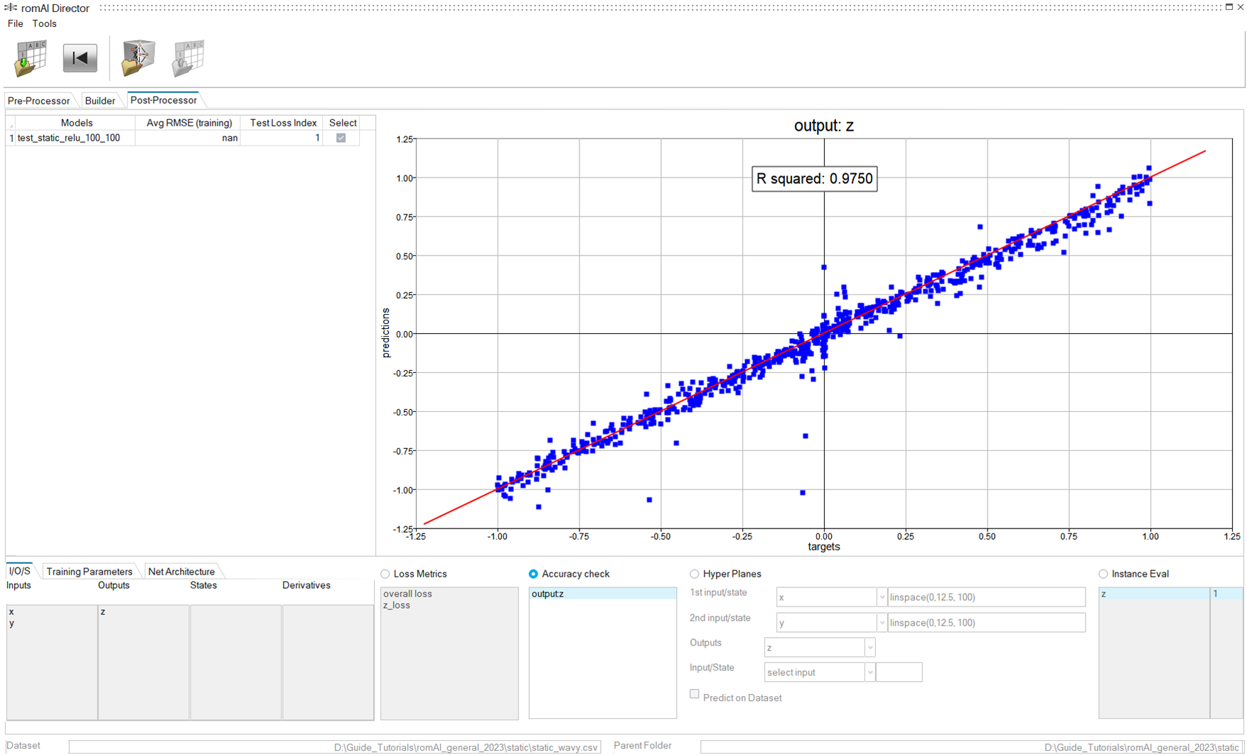
Accuracy check requires a test dataset for prediction. If the test dataset is not provided or if it incompatible with the model feature names, then an error dialog box is shown.
The test dataset name is populated in the file name info entries on the bottom of the panel.
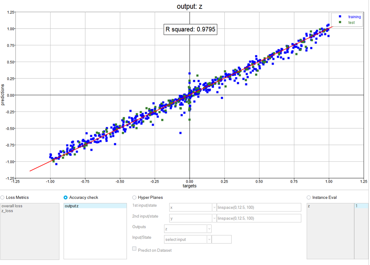
The training dataset is automatically loaded as test dataset in the post-processor just after the training. In this case, the training data points are shown with blue color and test data points are shown with green color.
The y-axis shows the predictions of the selected output produced by the romAI model, given the inputs defined in the dataset file.
The x-axis shows the targets for the same selected output contained in the same dataset file.
The closer that the predictions are to the targets, accordingly, more blue points will be aligned to the y = x curve, drawn in red.
The R2 coefficient gets computed automatically.
Define Hyper Planes
Select the Hyper Planes radio button.

- Hyper planes: The application evaluates the trained romAI model over a range of user-defined input values and displays the output as a hyper plane. One output at a time can be displayed.
- Scatter plots of Predictions vs Targets: The application evaluates the trained romAI model into a set of points contained in a dataset file and compares the output results with the target points contained in the same dataset file through a scatter plot. Only one output at a time can be requested.
Generate Hyper Planes
-
Select the 1st and 2nd inputs from the Inputs/States menu for the x-axis,
y-axis, and one output from the Outputs menu for the z-axis.
Figure 10. Inputs and Outputs Fields 
-
Specify the range of the x- and y-axes using Compose OML syntax.
Figure 11. Range of X- and Y-Axes 
The x/y grid is automatically created for the hyper plane. All other inputs and states are held constant.
-
For each additional input and state that you want to include, you can specify
the constant value for each through the menu and the slider.
Figure 12. Additional Input/State with Value Slider 
After you have specified the values for all the inputs and states, the hyper planes are updated automatically.
Figure 13. Updated Hyper Planes 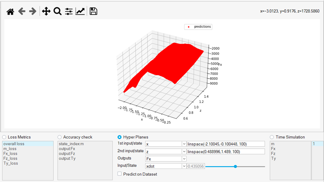
The axes are labeled with respect to the names of the selected inputs and states and output.
Generate Scatter Plots of Predictions vs Target
These plots require data from a dataset file.
-
To create Scatter Plots of Predictions vs Targets, select a test dataset
file.
Note: The format and labels used in the file are the same as the ones used for training. Otherwise, an error dialog box shows up.
-
Select the Predict on Dataset check box.
Note: The edit boxes, menu, and slider on the Hyper Planes panel are invisible in case of the Predict on Dataset option.
- Select the desired inputs and state variables from the Inputs/States box to create the x- and y-axes.
- Select the Outputs that you want to evaluate and compare.
-
Enter the Downsample Ratio.
The downsample value determines the number of points in the dataset file that will be used for the evaluation/comparison. For example:
- A downsample ratio of 1 means that the comparison between the romAI output and the target (contained in the dataset) will be performed for all the points in the dataset file.
- A downsample factor of 0.1 means that the comparison between the romAI output and the target (contained in the dataset) will be performed for a tenth of the points in the dataset file.
- When a dataset file is very large, adjusting the downsample ratio can greatly improve the plot performance. By default a downsample ratio value less than 1 is used on initial plots when the dataset is large.
Figure 14. Downsample Ratio of 1 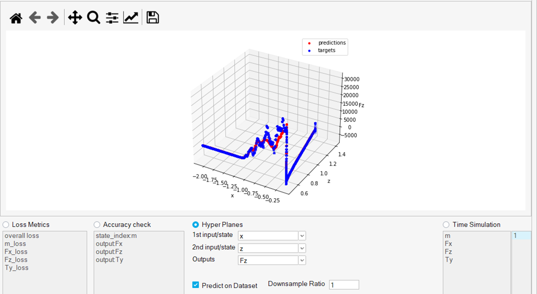
- To resume plotting hyper planes, deselect the Predict on Dataset check box.
Time Simulation Tab
If romAI is used to generate dynamic ROMs, it is important to have a tool that easily performs preliminary time simulations to assess the accuracy of the transient behavior after the romAI model has been trained.
The Time Simulation tab has been designed to perform these time simulations in just one step.
A time simulation is triggered. After the simulation runs successfully, the plot is updated.
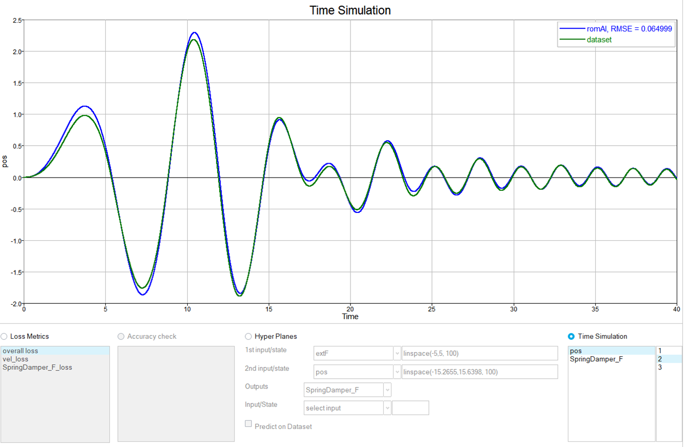
- Blue line: The dynamical results produced by the romAI model, given the inputs and the initial state conditions that are contained in the dataset file.
- Green line: The target time history.
- RMSE Metric: Root Mean Square Error calculated between the two signals is shown
in the legend. Note: The RMSE is calculated for the segment and output currently active.
Use the list box to select the output of the romAI model that you want to plot.
Compare Time Simulations of Several Models
The table of models lets you select several models to compare simulation results based on the same data inputs.

Instance Evaluation Tab
romAI can be used to generate static ROMs.
In this scenario, a time simulation is not meaningful, and it is replaced by a classical inference operation over the loaded dataset. Also, the tab name changes from “Time Sim” to “Instance Eval.”
Repeating the same steps as before, the following scatter plot is generated for a static ROM:

- Blue dots: The static results produced by the static romAI model, given the inputs contained in the dataset file.
- Green dots: the target results.
- RMSE Metric: Root Mean Square Error calculated between the romAI and dataset instances. Note: RMSE is calculated for the segment and output currently active.
Report Generation
The report generation tools can be accessed from Tools menu.
- Loss Metrics
- Accuracy Checks
- Time Simulation or Instance Evaluation
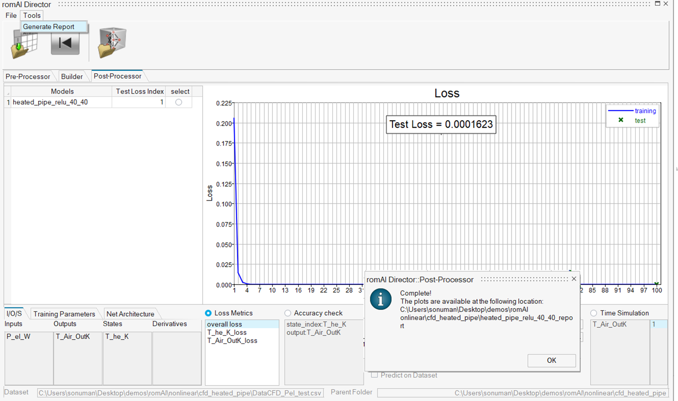
The report is saved in a folder with following syntax: <model_name>_report. Also, the folder location is displayed at the end of report generation.
FMU Export
The FMU export tool can be accessed from Tools menu.
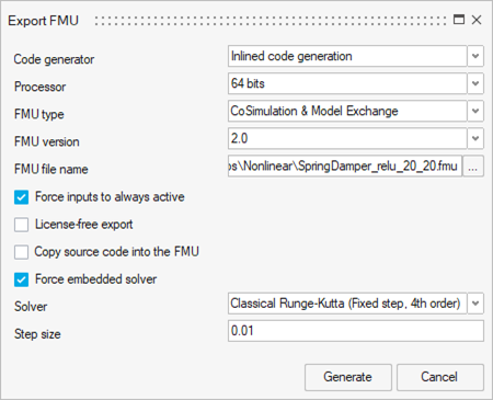
The parameters and options of the Export FMU dialog box are the same as in the Code Generation dialog with FMU selected as the target.
Two code generation technologies are available for selection: Standard code generation or Inlined code generation.
Both types of FMUs are supported: ME (Model Exchange) and CS (Co-Simulation).
Architecture (SINDy)
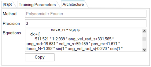
When you use the SINDy method, the Architecture tab contains the approximate system equation.
When you have created a model using the SINDy method, you automatically get access to the approximate system equation. You can copy the formula and reuse it from the Architecture tab.
Depending on the precision set, the coefficient is updated with the corresponding digits.
This feature is useful for creating smarter and more robust control system algorithms.
