SS-T: 3015 Imported Remote Loads on Specific Faces
Import and apply remote loads on specific faces.
- Purpose
- SimSolid performs meshless structural
analysis that works on full featured parts and assemblies, is tolerant of
geometric imperfections, and runs in seconds to minutes. In this tutorial,
you will do the following:
- Learn how to import/apply remote loads to specific faces on the model.
- Model Description
- The following model files are needed for this tutorial:
- RemoteLoadOnSpecificFaces.ssp
- RemoteLoadQuadcopter.csv
-
Figure 1. 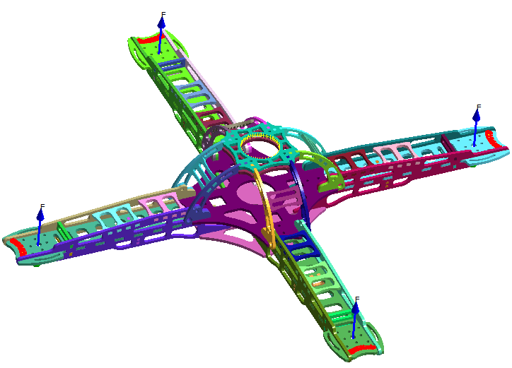
Open Project
- Start a new SimSolid session.
-
On the main window toolbar, click Open Project
 .
.
- In the Open project file dialog, choose RemoteLoadOnSpecificFaces.ssp
- Click OK.
Review Model
- In the Project Tree and modeling window, review the model.
-
Review connections.
Figure 2. 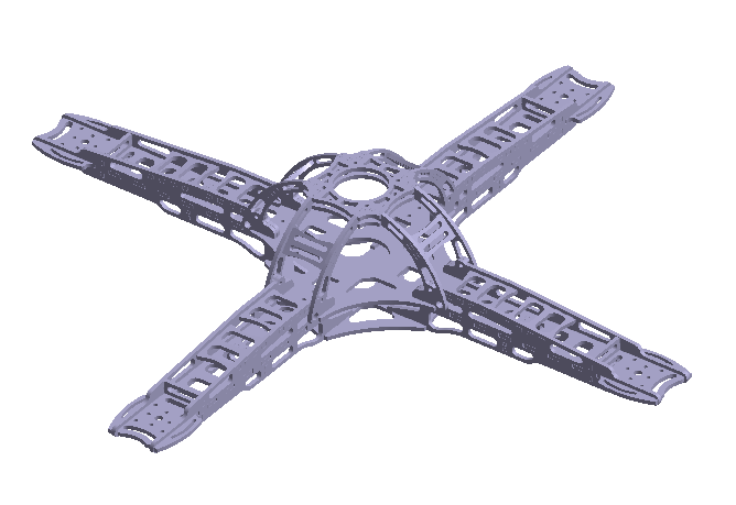
Create Multi-loadcase Analysis
-
On the main window toolbar, click Structural Analysis
 .
.
-
Select Multi-loadcases from the drop-down menu.
Figure 3. 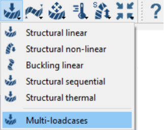
The workbench appears in the Project Tree.
Create Immovable Support
-
In the Multi-loadcase Workbench, click Immovable Support
 .
.
- In the dialog, verify the Faces radio button is selected.
-
In the modeling window, select the faces highlighted in
Figure 4.
Figure 4. 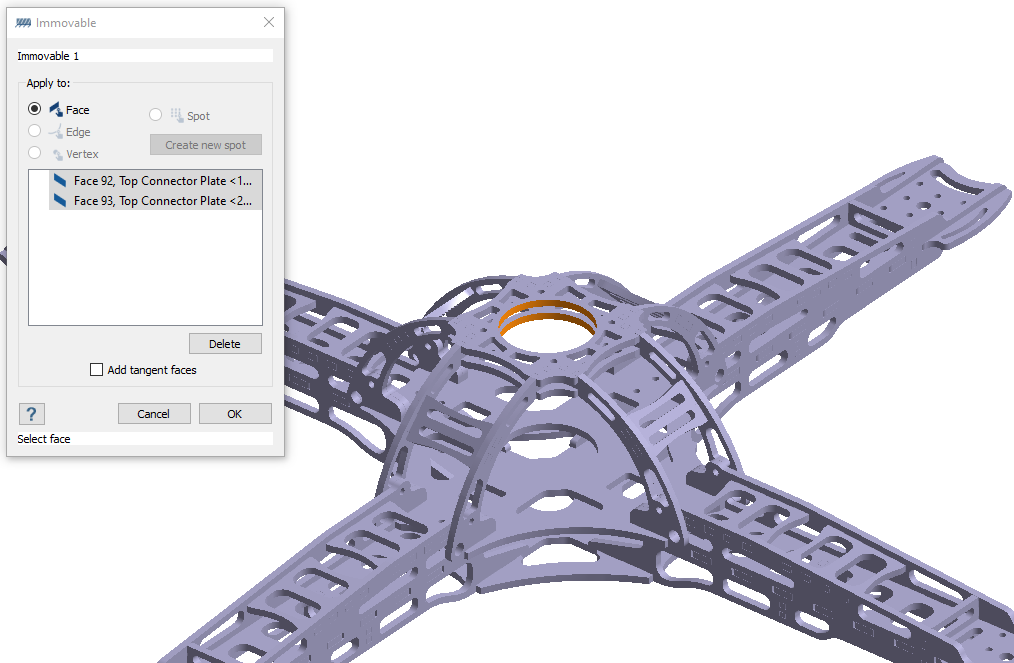
-
Click OK.
The new constraint, Immovable 1, appears in the Project Tree. A visual representation of the constraint is shown on the model.
Import Remote Load
-
On the workbench toolbar, select
 > Import remote loads.
- Set the coordinates to in.
- In the Imported remote load 1 dialog, click Import from CSV.
-
Select RemoteLoadQuadcopter.csv from the file explorer and
click Open.
The imported remote loads are shown in the dialog and mapped in the modeling window. You can edit the values in the dialog by clicking Edit Load or double-clicking on a row.
-
For Load Cases, choose a load case from the drop-down menu to view the desired
data.
By default, the coordinates and loads for Structural 1 are displayed.
Figure 5. 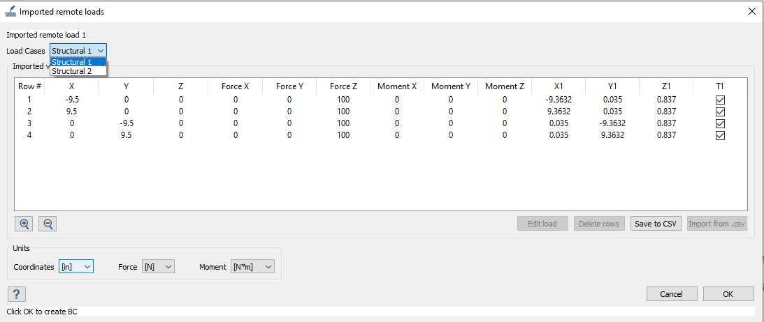
X1,Y1,Z1,T1,X2,Y2,Z2,T2 are optional fields and are used to define the faces to be mapped. These fields show up in the dialog only if they are defined.
For structural 1, X1, Y1, Z1 are the spatial coordinates of a point on the desired face to map the load.
-
Select the T1 check box to allow picking tangent
faces.
Figure 6. 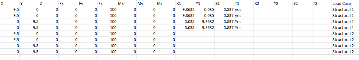
Structural 1 and Structural 2 have loads applied on the same remote point. In Structural 1, loads are applied on specified faces whereas Structural 2, mapping is based on remote point.Figure 7. 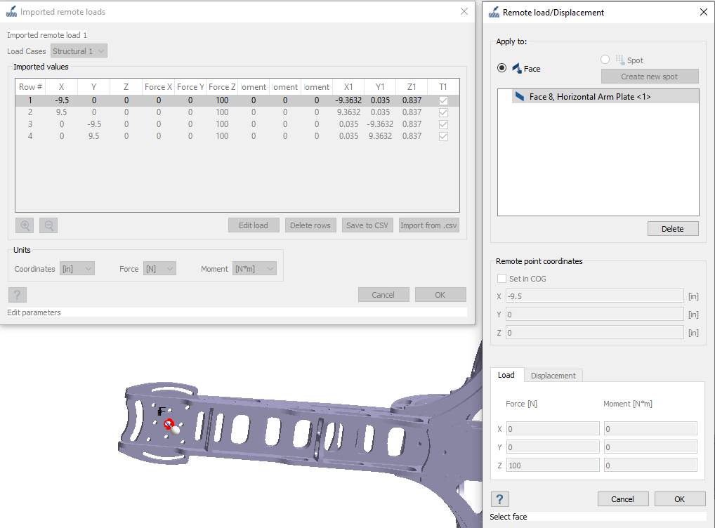
Figure 8. 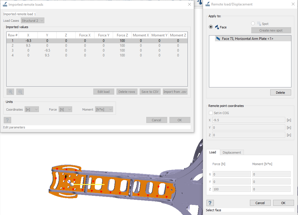
Edit Solution Settings
- In the Analysis branch of the Project Tree, double-click on Solution settings.
- In the Solution settings dialog, for Adaptation select Global+Local in the drop-down menu.
- Click OK.
Run Analysis
- On the Project Tree, open the Analysis Workbench.
-
Click
 (Solve).
Review Results
- In the Project Tree, select the analysis results branch.
-
On the Analysis Workbench toolbar, select
 (Result plot) > Displacement > Displacement Magnitude.
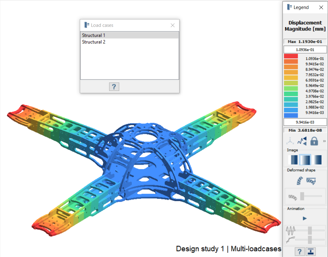
-
In the Load cases dialog, select the desired load case to
display the results.
Figure 9.