SS-T: 3020 Bearing Loads
Create bearing loads in SimSolid.
- Purpose
- SimSolid performs meshless structural
analysis that works on full featured parts and assemblies, is tolerant of
geometric imperfections, and runs in seconds to minutes. In this tutorial,
you will do the following:
- Learn how to create bearing loads in SimSolid.
- Model Description
- The following model file is needed for this tutorial:
- BearingLoads_Crankshaft.ssp
-
Figure 1. 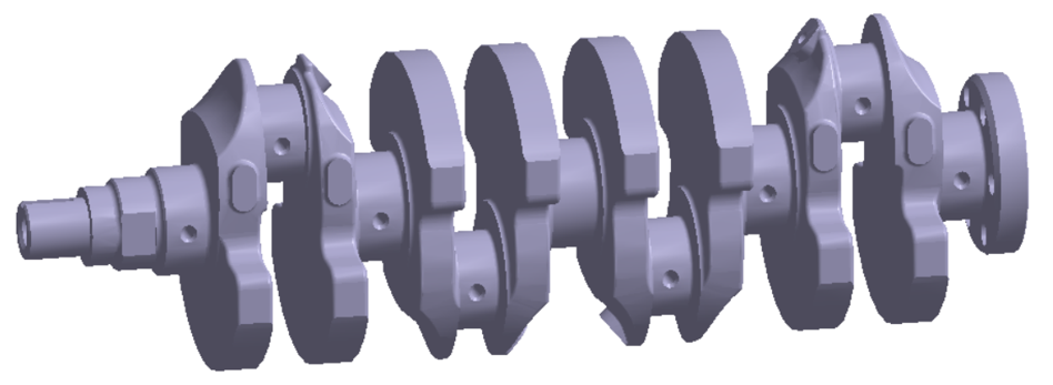
Open Project
- Start a new SimSolid session.
-
On the main window toolbar, click Open Project
 .
.
- In the Open project file dialog, choose BearingLoads_Crankshaft.ssp
- Click OK.
Create Structural Linear Analysis
On the main window toolbar, click Structural Analysis  > Structural linear.
The new analysis appears in the Project Tree
under Design study 1 and the Analysis Workbench
opens.
Create Immovable Support
-
In the Analysis Workbench, click Immovable
Support
 .
.
- In the dialog, verify the Faces radio button is selected.
-
In the modeling window, select the faces as highlighted
in the figure below.
Figure 2. 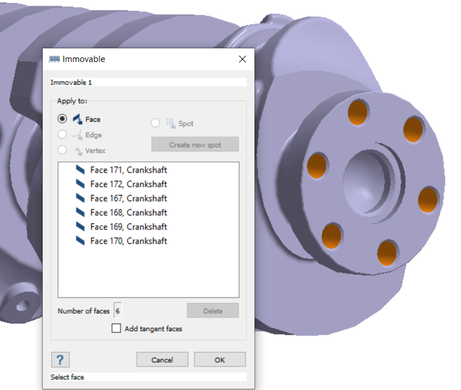
-
Click OK.
The new constraint, Immovable 1, appears in the Project Tree. A visual representation of the constraint is shown on the model.
Create Hinge Support
-
In the Analysis Workbench, click Immovable
Support
 .
.
-
In the dialog, select the other cylindrical face as highlighted in the figure
below.
Figure 3. 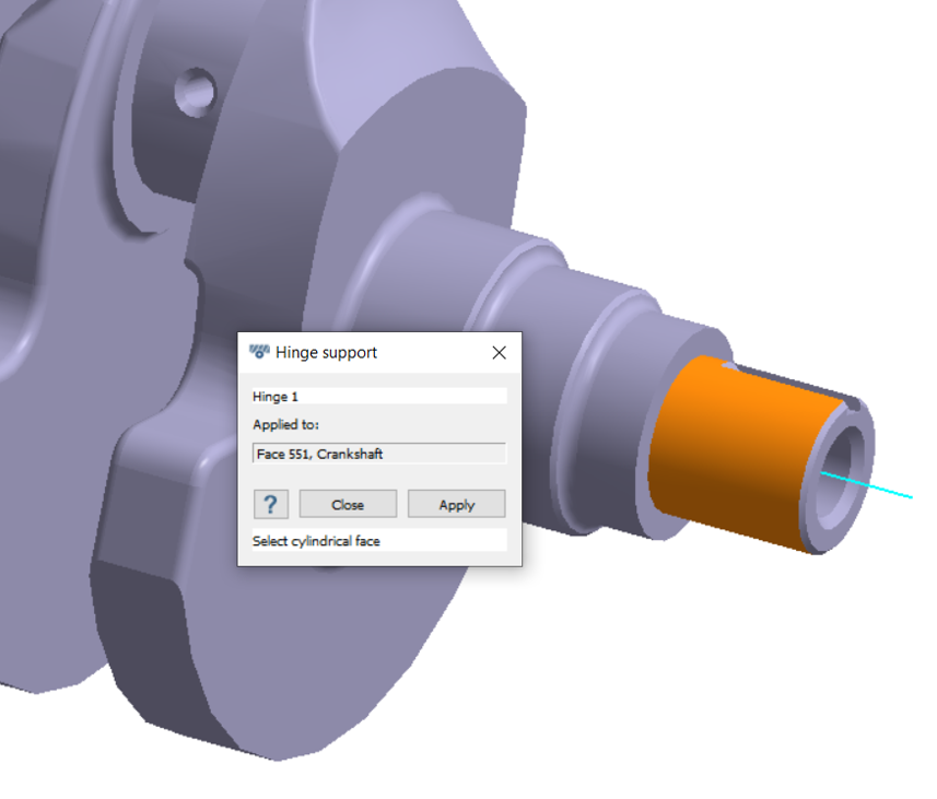
- Click Apply.
-
Click Close.
A new constraint, Hinge 1, appears in the Project Tree.
Apply Bearing Load
-
On the Analysis Workbench toolbar, click
 (Bearing loads).
-
In the modeling window, select faces as shown in Figure 4.
Figure 4. 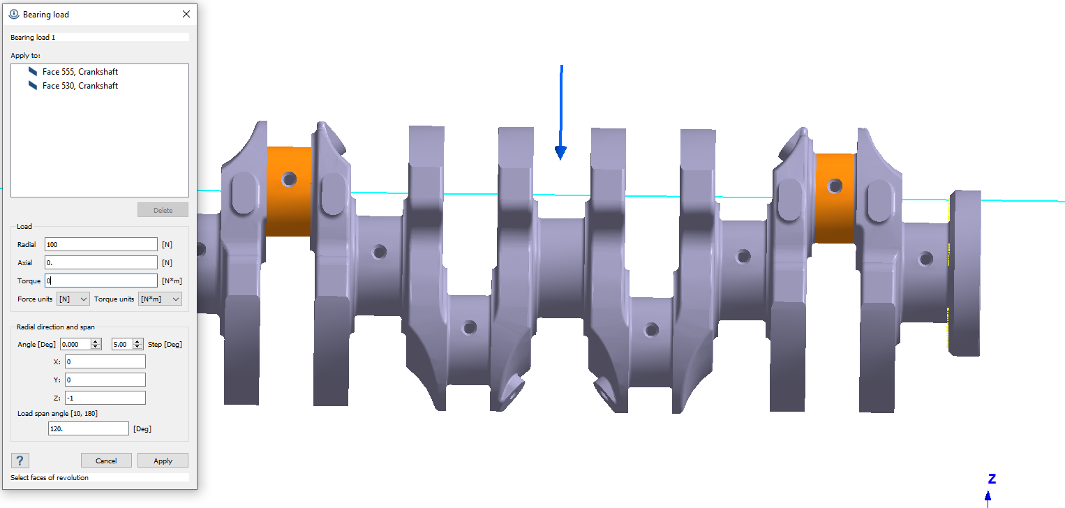
- For Load, enter 100 in the Radial direction.
-
Under Direction, for X enter 0.00000, for Y enter
0.00000, and for Z enter
-1.00000.
Tip: You can also edit Direction by using the slider bar, the spin wheel, or by entering the angle.
- For Load span and angle, enter 120.
- Click Apply.
-
Repeat steps 1 through 6 by selecting the faces shown in Figure 5
Figure 5. 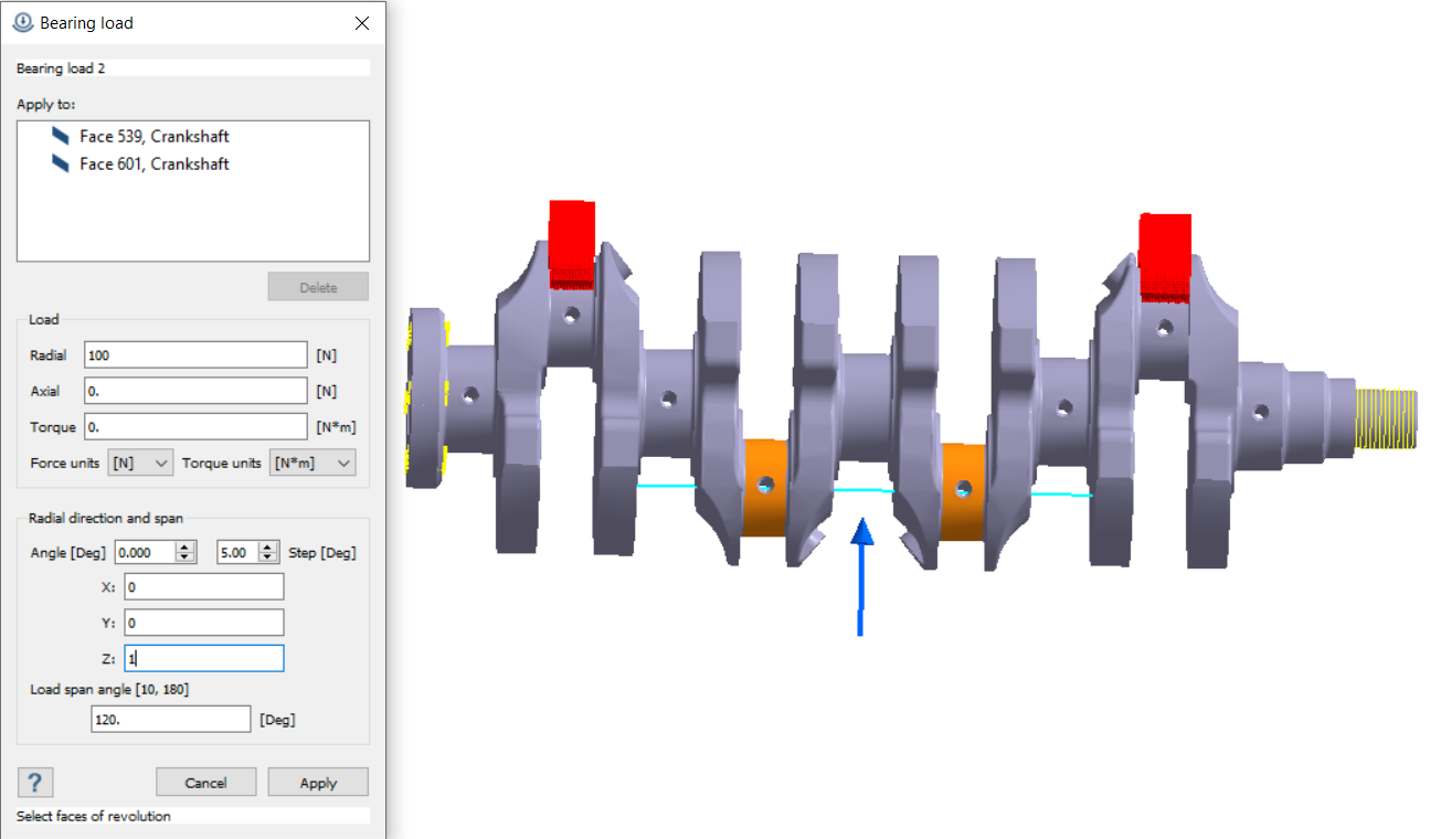
- Under Direction, for X enter 0.00000, for Y enter 0.00000, and for Z enter 1.00000.
- Click Apply.
- Click Cancel.
Edit Solution Settings
- In the Analysis branch of the Project Tree, double-click on Solution settings.
- In the Solution settings dialog, for Adaptation select Global+Local in the drop-down menu.
- Click OK.
Run Analysis
- On the Project Tree, open the Analysis Workbench.
-
Click
 (Solve).
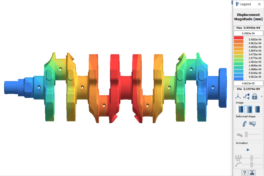
Review Results
-
On the Analysis Workbench
toolbar, click
 (Results plot).
-
Select Displacement Magnitude.
The Legend window opens and displays the contour plot.
Figure 6.