
RD-V: 0240 Tabulated Material (LAW36)
The analysis shows the behavior of the tabulated material /MAT/LAW36 under tensile load-cases.
Options and Keywords Used
Input Files
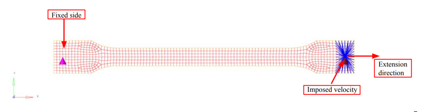
Model Description
Units: Kg, mm, ms, GPa
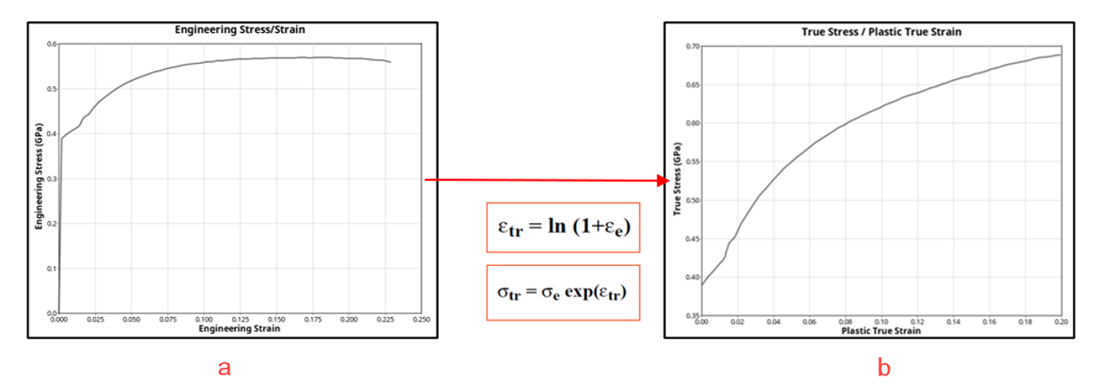
Material Law Characterization
- Material Property
- Value
- Young's modulus
- 221 GPa
- Poisson ratio
- 0.3
- Thickness
- 1.7mm
Results
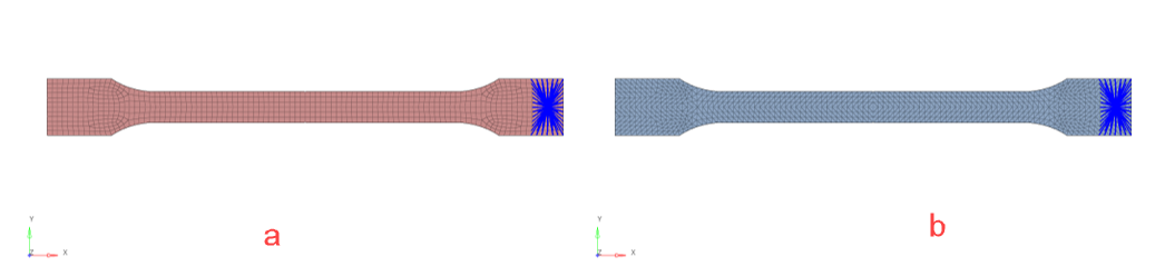
Tensile Coupon with Shell Elements
- /PROP/TYPE1 (SHELL), QEPH shell formulation Ishell=24, 5 integration points through thickness. Figure 4 shows the results of the plastic strain contour. Here, the beginning of striction can be observed.
Figure 4. Plastic strain contour plot for shell QEPH shell formulation 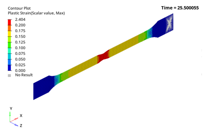
In Figure 5, the true stress versus true strain curve is directly extracted from an instrumented element at the center of the coupon.
The engineering stress versus engineering strain curve is calculated globally with the following steps:- The engineering stress can be calculated by using σe= F/A0. The force is derived from the rigid body force. The original cross-sectional area is 20.4 mm2.
- The engineering strain is calculated with . The elongation is measured from two instrumented nodes. The original distance l0 is 80 mm.
Figure 5. Comparison of results using LAW36 for shell QEPH shell formulation 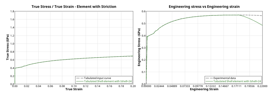
The simulated true stress versus true strain curve matches perfectly the corresponding experimental curve. The simulated engineering stress versus engineering strain curve matches perfectly the corresponding experimental curve until striction starts at which point effort starts to decrease.
- /PROP/TYPE1 (SHELL) QBAT shell formulation Ishell=12, 5 integration points through thickness Figure 6 shows the results of the plastic strain contour. The beginning of striction can be observed.
Figure 6. Plastic strain contour plot for shell QBAT shell formulation 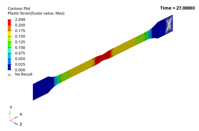
Figure 7. Comparison of results using LAW36 for shell QBAT formulation 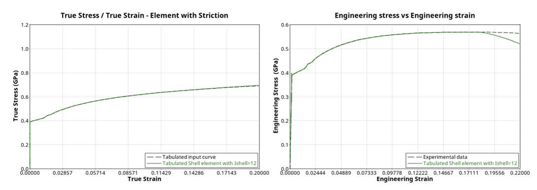
The simulated true stress versus true strain curve matches perfectly the corresponding experimental curve. The simulated engineering stress versus engineering strain curve matches perfectly the corresponding experimental curve until striction starts at which point effort starts to decrease.
Tensile Coupon with SH3N Elements
- Ish3n = 0Figure 8 shows the results of the plastic strain contour plot visualization. The beginning of striction can be observed.
Figure 8. Plastic strain contour plot for sh3n element 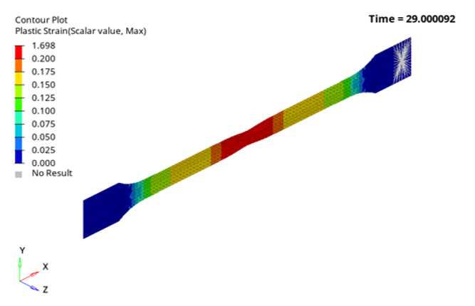
Figure 9. Comparison of results using LAW36 for SH3N element 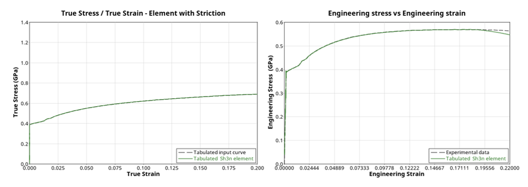
The simulated true stress versus true strain curve matches perfectly the corresponding experimental curve. The simulated engineering stress versus engineering strain curve matches perfectly the corresponding experimental curve until striction starts at which point effort starts to decrease.
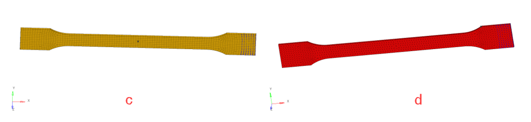
Tensile Coupon with Solid Hexahedron Elements
- /PROP/TYPE14 (SOLID), Isolid =24Figure 10 shows the results of the plastic strain contour plot visualization. The beginning of striction can be observed.
Figure 10. Plastic strain contour plot for solid element 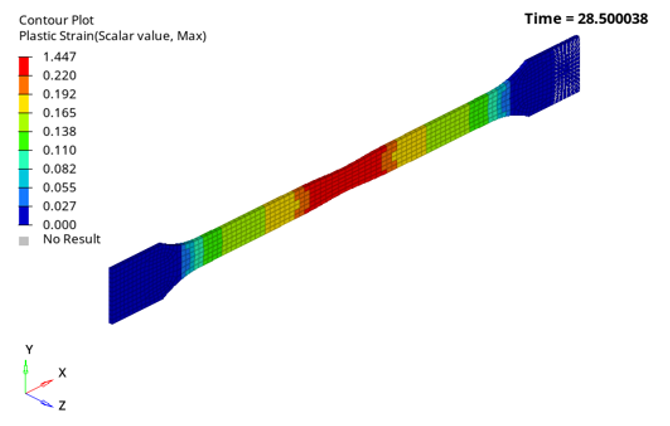
Figure 11. Comparison of results using LAW36 for solid element 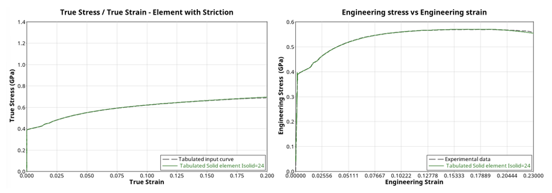
The simulated true stress versus true strain curve matches perfectly the corresponding experimental curve. The simulated engineering stress versus engineering strain curve matches perfectly the corresponding experimental curve until striction starts at which point effort starts to decrease.
- /PROP/TYPE14 (SOLID), Isolid =18Figure 12 shows the results of the plastic strain contour plot visualization. The beginning of striction can be observed.
Figure 12. Plastic strain contour plot for solid element 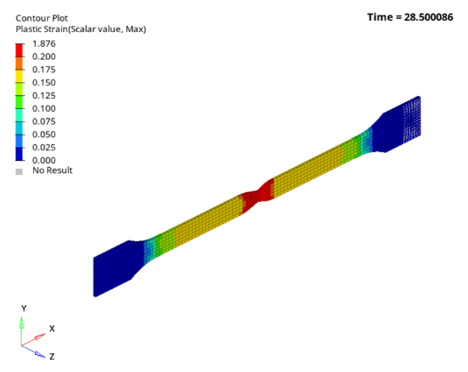
Figure 13. Comparison of results using LAW36 for solid element 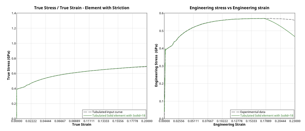
The simulated true stress versus true strain curve matches perfectly the corresponding experimental curve. The simulated engineering stress versus engineering strain curve matches perfectly the corresponding experimental curve until striction starts at which point effort starts to decrease.
Tensile Coupon with Thick Shell Elements
- /PROP/TYPE20 (TSHELL), Isolid =15Figure 14 shows the results of the plastic strain contour plot visualization. The beginning of striction can be observed.
Figure 14. Plastic strain contour plot for TShell element 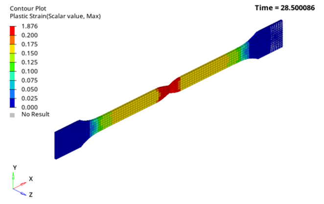
Figure 15. Comparison of results using LAW36 for TShell element 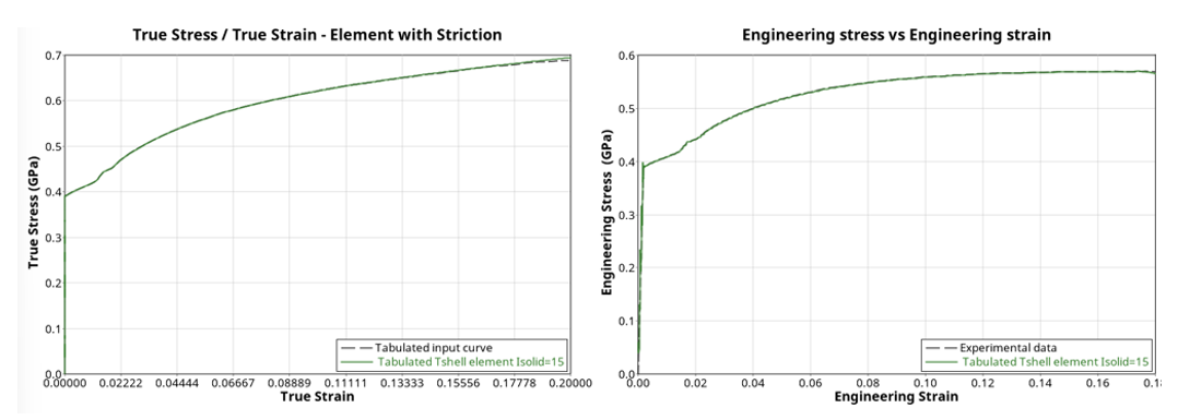
The simulated true stress versus true strain curve matches perfectly the corresponding experimental curve. The simulated engineering stress versus engineering strain curve matches perfectly the corresponding experimental curve until striction starts at which point effort starts to decrease.
Tensile Coupon with Solid Tetrahedron Elements
- /PROP/TYPE14 (SOLID), Itetra4=0Figure 16 shows the results of the plastic strain contour plot visualization. As can be seen at the end of simulation the striction is barely initiated. This is due to the very stiff element formulation.
Figure 16. Plastic strain contour plot 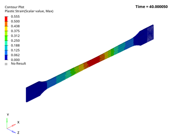
Figure 17. Comparison of results using LAW36 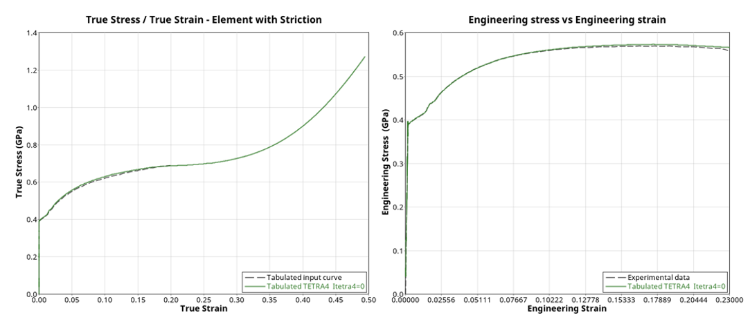
The simulated true stress versus true strain curve matches perfectly the corresponding experimental curve. After this point, the stress continues to increase, in contrast to other results presented previously. The simulated engineering stress versus engineering strain curve matches perfectly the corresponding experimental curve until striction starts at which point effort starts to decrease.
- /PROP/TYPE14 (SOLID), Itetra4=3
Figure 18 shows the results of the plastic strain contour plot visualization. Using Itetra4=3, the striction can be observed in contrast to the formulation above (with Itetra4=0).
Figure 18. Plastic strain contour plot 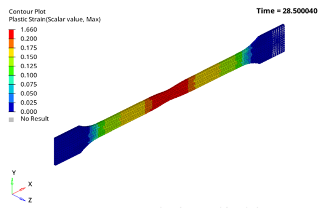
Figure 19. Comparison of results using LAW36 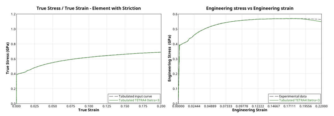
The simulated true stress versus true strain curve matches perfectly the corresponding experimental curve. The simulated engineering stress versus engineering strain curve matches perfectly the corresponding experimental curve until striction starts at which point effort starts to decrease.
- /PROP/TYPE14 (SOLID), Itetra10=0Figure 20 shows the results of the plastic strain contour plot visualization. You can spot the beginning of striction.
Figure 20. Plastic strain contour plot 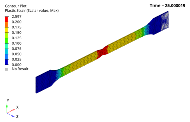
Figure 21. Comparison of results using LAW36 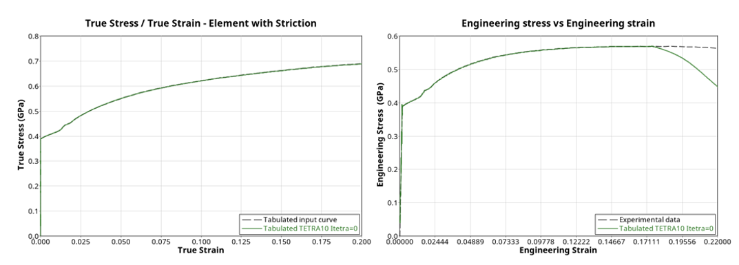
The simulated true stress versus true strain curve matches perfectly the corresponding experimental curve. The simulated engineering stress versus engineering strain curve matches perfectly the corresponding experimental curve until striction starts at which point effort starts to decrease.
- /PROP/TYPE14 (SOLID), Itetra10=2Figure 22 shows the results of the plastic strain contour plot visualization.
Figure 22. Plastic strain contour plot 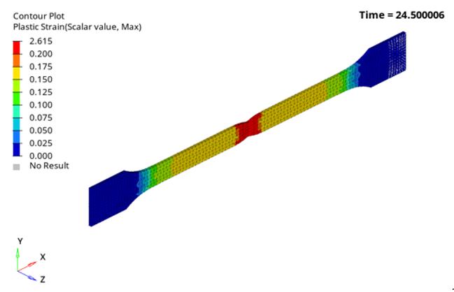
Figure 23. Comparison of results using LAW36 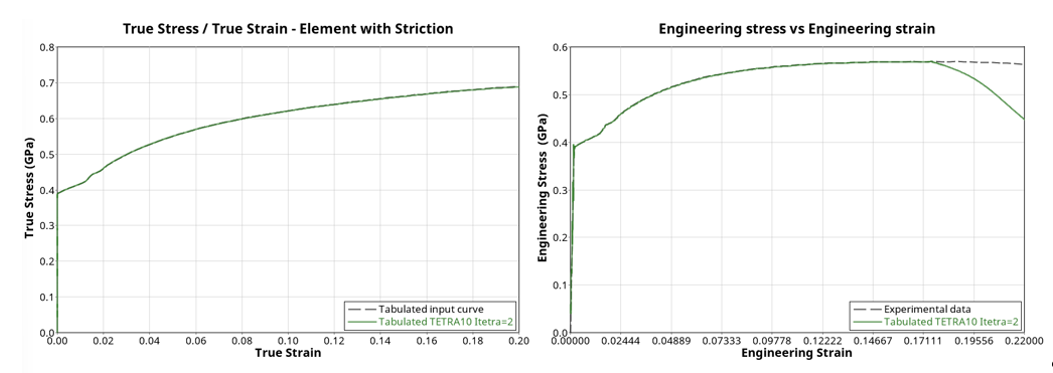
The simulated true stress versus true strain curve matches perfectly the corresponding experimental curve. The simulated engineering stress versus engineering strain curve matches perfectly the corresponding experimental curve until striction starts at which point effort starts to decrease.
Conclusion
The materiel LAW36 was used with experimental data for different element to compare with simulations data. The simulation results of stress-strain curves overlay perfectly with input experimental curves for all element formulations evaluated.
| Model | Parameter | Relative Cost |
|---|---|---|
| Shell | Ishell=24 | 1 |
| Ishell=12 | 1.64 | |
| Sh3n* | Ish3n=0 | 2.17 |
| Model | Parameter | Relative Cost |
|---|---|---|
| Hexahedron | Isolid=24 | 1 |
| Isolid=18 | 1.17 | |
| Isolid=15 | 1.07 |
| Model | Parameter | Relative Cost |
|---|---|---|
| Tetrahedron | Itetra4=0 | 1 |
| Itetra4=3 | 1.3 | |
| Itetra10=0 | 14.07 | |
| Itetra10=2 | 7.71 |