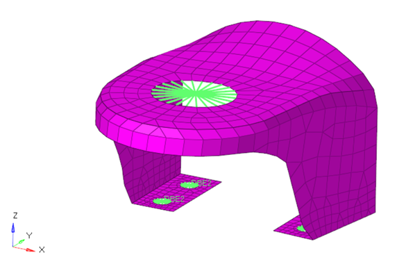
A bracket tested for frequency response analysis is utilized to perform the Sine
Sweep Fatigue Analysis. The model is already setup for the FRF analysis, an
additional loadstep for SN-Fatigue Calculation is created in this tutorial. The FRF
subcase will be utilized for the fatigue calculation, and a
TABLED card scaling the same.
Note: The sweep parameters are
currently supported by editing the .fem deck generated,
which is explained in this tutorial.
Figure 1. bracket_frf Model for Fatigue Analysis
Launch HyperMesh and Set the OptiStruct User Profile
Launch HyperMesh.
The User Profile dialog opens.
Select OptiStruct and click
OK.
This loads the user profile. It includes the appropriate template, macro
menu, and import reader, paring down the functionality of HyperMesh to what is relevant for generating models for
OptiStruct.
Import the Model
Click File > Import > Solver Deck.
An Import tab is added to your tab menu.
For the File type, select OptiStruct.
Select the Files icon .
A Select OptiStruct file browser
opens.
Select the bracket_frf.fem file you saved
to your working directory.
Click Open.
Click Import, then click Close to
close the Import tab.
The outline of the Fatigue Analysis setup to be achieved in the following
steps.Figure 2. Fatigue Setup Sine Sweep – SN Damage
Set Up the Model
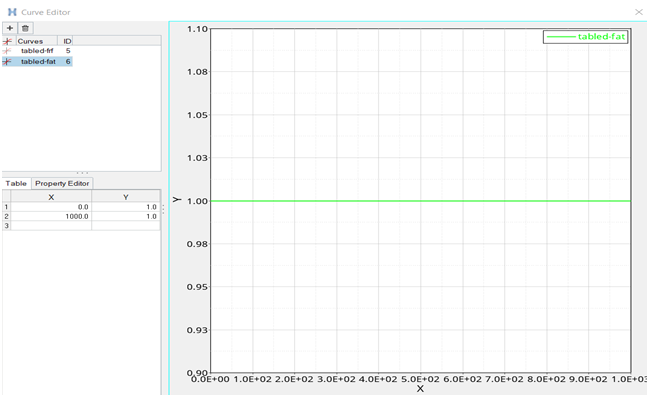
Create TABLED1 Curve
For Sine Sweep Fatigue Analysis, the TABLEDx card is used in place of TABFAT.
In the Model Browser, right-click and select Create > Curve.
For Name, enter tabled-fat.
Enter the following magnitudes for (x,y).
In the x1 field, enter 0.0
In the y1 field, enter 1.0
In the x2 field, enter 1000.0
In the y2 field, enter 1.0
Close the Curve Editor window.
In the Model Browser under Curves, select
tabled-fat.
For Card Image, select TABLED1 from the drop-down menu.
Set XAXIS and YAXIS interpolation scheme to
LINEAR.
Figure 3. TABLED1 Curve
Click Close.
The load collector TABLED1 that defines the time history of the
loading has been created.
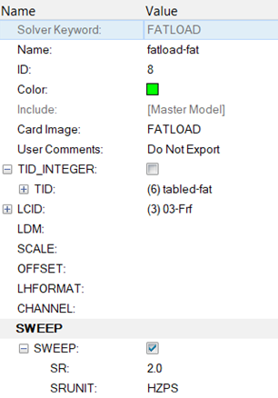
Define FATLOAD Load Collector
The model has a Frequency Response loadstep defined, which is
used to define the FATLOAD.
In the Model Browser, right-click and select Create > Load Collector.
For Name, enter fatload_fat.
For Card Image, select FATLOAD.
Select the option for TID INTEGER.
Set the TID value as the curve ID of tabled-fat (8 in this tutorial).
For LCID(load case ID), select 03_frf from
the list of load steps.
Note: TABFAT and scaling parameters are not required for this
calculation.
Select the Option for SWEEP and define the sine sweep
parameters via SR (sweep rate) and SRUNIT
(sweep rate unit) fields.
Figure 4. FATLOAD with LCID and SWEEP Parameters
Define FATEVNT Load Collector
Create a random response event for the
FATLOAD_RAND created.
In the Model Browser, right-click and select Create > Load Collector.
For Name, enter fatevent-fat.
For Card Image, select FATEVNT.
For FATEVNT_NUM_FLOAD, enter 1.
Select fatload-fat for FLOAD in
the Loadcol field.
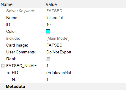
Define FATSEQ Load Collector
In the Model Browser, right-click and select Create > Load Collector.
For Name, enter fatseq-fat.
For Card Image, select FATSEQ.
For FATSEQ_NUM enter 1, as 1 FATEVENT has been
created.
For FID (Fatigue Event Definition), select fatevent-fat and N as
1.
Figure 5. FATSEQ showing fatevent-fat created
Defining the sequence of events for the fatigue analysis is completed.
The Fatigue parameters are defined next.
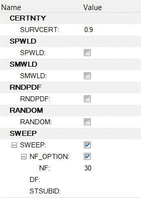
Define Fatigue Parameters
In the Model Browser, right-click and select Create > Load Collector.
For Name, enter fatparm-fat.
For Card Image, select FATPARM.
Verify TYPE is set to SN.
Set STRESS COMBINE to VONMISES.
Set STRESSU to MPA (Stress Units).
Set CERTNTY SURVCERT to 0.9.
Select the SWEEP option and define
NF=30.
Figure 6. FATPARM with SWEEP Parameters
Define Fatigue Material Properties
The material curve for the fatigue analysis can be defined on the
MAT1 card.
In the Model Browser, click on the MAT1 material.
The Entity Editor opens.
In the Entity Editor, set MATFAT to SN.
Set UTS (ultimate tensile stress) to 340.0.
Set YS (yield strength) to 180.0.
For the SN curve set (these values should be
obtained from the material's SN curve):
SRI1
936.0
B1
-0.161907
NC1
1e20
FL
1.0
SE
1.0
Define PFAT Load Collector
In the Model Browser, right-click and select Create > Load Collector.
For Name, enter pfat-fat.
For Card Image, select PFAT.
Set LAYER to WORST.
Set FINISH to NONE.
Set TRTMENT to NONE.
Set Kf to 1.0.
Define FATDEF Load Collector
In the Model Browser, right-click and select Create > Load Collector.
For Name, enter fatdef-fat.
Set the Card Image to FATDEF.
Activate PTYPE and PSHELL in
the PTYPE Entity Editor.
Edit FATDEF_PSOLID_NUMIDS to 1.
Select new_bracket for PID and pfat-fat for PFATID.
Define the Fatigue Load Step
In the Model Browser, right-click and select Create > Load Step.
For Name, enter 04-Fatigue.
Set the Analysis type to fatigue.
For FATDEF, select fatdef-fat.
For FATPARM, select fatparm-fat.
For FATSEQ, select fatseq-fat.
Submit the Job
From the Analysis page, enter the OptiStruct
panel.
Click save as following the input file field.
The Save As dialog opens.
For File name, enter the name bracket-frf.fem.
Click Save.
Click OptiStruct to submit
the analysis.
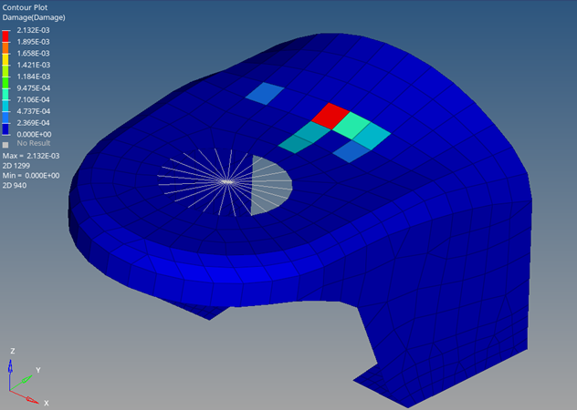
Review the Results
From the OptiStruct panel, click HyperView.
HyperView is launched and the results are
loaded. A message window appears to inform of the successful model and result
files loading into HyperView.
Go to the Results tab.
In the Results tab, select Subcase 4
(04-Fatigue) from the subcase field.
On the Results toolbar, click to open the
Contour panel.
Set Result type to Damage and click on
Apply to contour the elements.

 .
A Select OptiStruct file browser opens.
.
A Select OptiStruct file browser opens.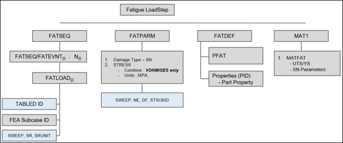
 to open the
Contour panel.
to open the
Contour panel.