Transfer Path Analysis

Transfer Path Analysis (TPA) is used to estimate and rank the noise or vibration contributions via the different structural transmission paths in a system.

The function of the TPA is to determine which body interface dominates the critical NVH response in the interior of the body for a given type of vehicle loading. The calculation involves the Transfer function, Point Mobility, Grid points force and Path participation.

Figure 1.

(1)

X_{t} = \sum_{p a t h s} [X_{i}] = \sum_{p a t h s} [{(\frac{X}{F})}_{i} * F_{i}]

Where,

$X_{i}$: Acoustic or Structural Response at a certain location
$X_{i}$: Contribution from path $i$
${(\frac{X}{F})}_{i}$: Acoustic or Structural Transfer Function for path $i$
$F_{i}$: Attachment Force through path $i$

Setup and Run

Typical Transfer Path Analysis in simulation requires two steps.

Two Step Setup

Calculate attachment force of the system in an assembled state:
- Assemble the system together for example, a full vehicle model and identify the responses (acoustic or structural) for which TPA analysis will be performed. Typical acoustic response is the grid at the approximate Driver’s Ear location. An example of structural response would be steering wheel response point where the driver would place their hands.
- Identify all the attachment points through which loads may be transferred from the excited structure (Powertrain and Chassis in Figure 1) to the responding structure (the Body in the picture above). Each degree of freedom (dof) at the attachment point becomes a transfer path.
- Setup a Frequency Response Analysis to calculate the forces acting on the attachment dofs, as well as the acoustic/structural responses (identified in step i above). The acoustic/structural responses calculated by the solver are compared to the acoustic/structural response constructed summing up the paths as shown in Equation 1.
Calculate Transfer Functions (TF) of the responding structure in an isolated state:
- Break the system at the attachment points, and perform Free Body Analysis with the responding structure isolated, as if it is not connected to the excited structure.
- Calculate the cross transfer functions (Tactile Transfer Function for the structural response grid and Acoustic Transfer Function for the acoustic response grid) between the attachment points to the response grids, as well as driving point transfer functions (that is, Point Mobility), by applying a unit load to each attachment dof as shown in Figure 2.
  
  Figure 2. Calculation of Transfer Functions and Point Mobility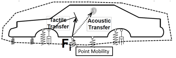

Automated TPA Process (One Step TPA)

A simplified process has been developed in OptiStruct that allows the necessary data needed for the TPA analysis to be requested (using PFPATH card) in a single frequency response analysis run, where the transfer functions and attachment forces are output to a single H3D file.

The traditional TPA involves 2 solver runs (as shown in Setup and Run) and needs the subcases labeled properly to allow for automatic assignment of path details in the TPA post-processing utility available in NVH utilities in HyperView.

Once the resulting H3D file is loaded into the TPA utility in HyperView, transfer function results are automatically matched up with the attachment forces results. This automated TPA process significantly improves the efficiency and robustness of the TPA analyses.

Setup

With One Step TPA, you do not need to worry about setting up the multiple subcases as would be required for Two Step TPA since you would need to setup a subcase per Attachment Point per dof for the Transfer Function analysis run. Also, with Two Step TPA, you will have to label these subcases very carefully for the TPA utility to allow automated path assignment.

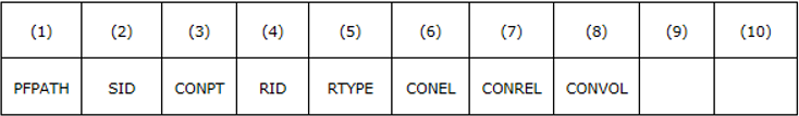
To setup One Step TPA, all you need to do is to add the PFPATH Bulk Data Entry and reference it using the PFPATH I/O Option Entry of the FEM file for an existing Frequency Response Run. PFPATH is supported for both Modal and Direct Frequency Response Analysis. PFPATH support Force as well as Enforced Displacement, Velocity and Acceleration as input. Shown below are the different fields of the PFPATH Bulk Data Entry.

Required Data for PFPATH:

CONPT: The connection points with a SID of type GRID SET.
RID: The response SID of type GRIDC. Contribution to each response DOF through the connection points will be calculated.
RTYPE: Criterion for the type of response; the response type corresponding to a structural dof could be displacement (DISP), velocity (VELO) or acceleration (ACCE). For pressure on fluid grid, the type is DISP.

Optional Data for PFPATH:

CONEL: The ELEMENT set consists of elements connected to the connection GRIDs in CONPT.; These elements represent connecting paths from the rest of the system to the user-defined control volume.
CONREL: The RIGID set consist of rigid elements, connected to the connection GRIDs in CONPT.; These rigid elements represent connecting paths from the rest of the system to the user-defined control volume.
CONVOL: The GRID set consists of the grids used to define the control volume.; If CONVOL is not specified, OptiStruct will export a file called, <filename>_outsidecv.fem, which contains a list of all grids outside the control volume. This file can be imported into HyperMesh to visualize the grids outside the control volume.

Example

*.fem file showing the usage of the PFPATH card.

PFPATH=1
$$------------------------------------------------------------------------------$
$$                      Case Control Cards                       		  $
$$------------------------------------------------------------------------------$
SUBCASE 1 
   DLOAD=10
   FREQ = 2
   METHOD = 1
…
BEGIN BULK
PFPATH,1,100,10,DISP
.
.
…
ENDDATA

Result Files

The TPA utility in HyperView requires 2 result files.

Two Step TPA

The Transfer Function output file contains the cross transfer function results between the attachment dofs and the response grids for which TPA analysis is desired. Optionally and preferably, driving Point Mobility (PM) results are also available in this file and allow you to examine local stiffness attachment effects.

The Force output file containing the attachment forces and the Total Responses for the Response Grids, for which TPA is being done. It is assumed that the forces are output using a local co-ordinate system (LCS) aligned with the one used for the TF output. The easiest way to ensure consistency is to use the GPFORCE output request using OptiStruct.

Table 1. Common Force Requests
Force Request Type	Output LCS	Comment
GPFORCE	Grid analysis LCS	Same as force input LCS
ELFORCE	Element LCS	May differ from the input LCS
SPCFORCE	Grid analysis LCS	Same as force input LCS

For a Two Step TPA, there will be 2 separate result files, one containing the Transfer Function (and optionally the Point Mobility results) and the second containing the attachment forces and the Total Response for the Response grids for which TPA is being done.

For One Step TPA, all the results (Transfer Functions, Point Mobilities, Attachment Forces, Total Response(s)) are in one H3D file.

When analyzing Two Step TPA results, if the subcase labeling convention (given below) is followed, it allows for automated assignment of path details by the TPA utility.

TF Subcase Labeling Convention

Excited Grid ID:DoF<>Connector Element ID:DoF<>L1:L2:L3:DoF

Where, L1, L2, and L3 are levels of description for an attachment point that are used to aggregate path contributions.

Example

4003003:+X<>3003:+X<>Frt Susp.:LCA - Frt Bush:LHS:+X

Where,

4003003:+X: Is a basic descriptor of the path and provides the excited Grid ID and DoF.
<>: Is a delimiter between parts of the label.
Frt Susp.:LCA - Frt Bush:LHS:+X: Provides a more meaningful description for the attachment point and DoF.

Any and all parts of the label may be missing from the TF subcase label, but the more complete the label is, the less it needs to be manually filled in to sufficiently define path information needed for the analysis.

Scenarios of TF Subcase Labels

No label or unexpected label.
The Utility makes all TF subcases available in the Path Details dialog so that you can add transfer paths manually in the Point tab and assign the proper subcase to each path in the TF tab.
Label includes only Part 1 - Excited Grid ID: DoF.
The Utility builds a list of transfer paths in the Point tab, and assign the labeled subcase to the corresponding path in the TF tab. You will need to manually assign forces to the paths in order to proceed with the analysis
Label includes Part 1 and Part 2 - Connector Element ID: DoF.
The Utility builds a list of transfer paths in the Point tab, and assign the labeled subcase to the corresponding path in the TF tab, and assign force data matching the Grid and/or Element ID to the proper path in the Force tab.
Label includes all three parts.
The Utility builds a list of transfer paths and adds proper descriptions to the attachment point in the Point tab, assigns the labeled subcase to the corresponding path in the TF tab, and assigns force data matching the Grid and/or Element ID to the proper path in the Force tab.

One Step TPA

All the results (Transfer Functions, Point Mobilities, Attachment Forces, Total Response(s)) are in one H3D file. Once the resulting H3D file is loaded into the TPA utility, TF results are automatically matched up to the attachment forces results that are guaranteed to be consistent in terms of co-ordinate systems being used for TF and attachment forces. This significantly improves the efficiency and robustness of the TPA analyses.

Post-processing

Post-process using the TPA utility in HyperView.

Launch the Transfer Path Analysis utility from the NVH menu in HyperView, or select File > Load > Preference File.
The Preferences dialog is displayed as shown in Figure 4.

Figure 4. Loading the NVH Menu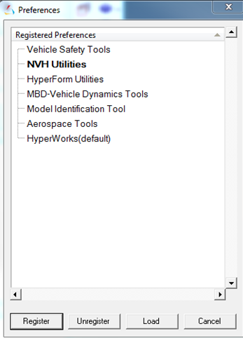
Select NVH Utilities.
Click Load.
In the Load tab, point to the result files containing the Transfer Function results and the Force (attachment forces) results.
For Two Step TPA, these will be 2 different files but for One Step TPA it will be one h3d file containing TF and attachment forces results.
Click Load.
The Path Details dialog will populate automatically for One Step TPA. The Path Details will be populated automatically for Two Step TPA if the subcase naming convention is followed as discussed in previous section.

Figure 5. Load Tab of TPA Utility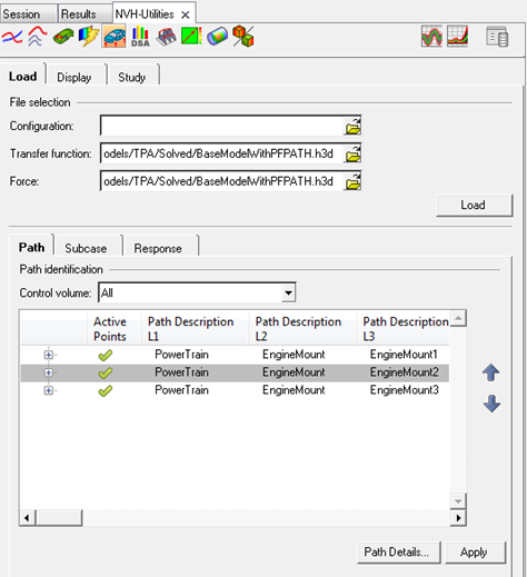
Click Path Details to confirm if all the paths have been accounted for.
Click Close.
In the Path tab, click Apply.

Figure 6. Path Details Window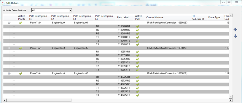
On the Subcase tab, select the frequency response subcases listed, and click Apply.
On the Response tab, select the Subcase, Result type, Response ID and Direction component.

Tip: You can also provide a Response label for the Response ID. If you need to see the plots for each dof for all the attachment points, toggle the option Generate all path contribution plots.
Click Load Response.
Note: The Calculated Response which is the summation of all the paths (RHS of EQ 1) is plotted against the Response calculated by the Solver as shown in Figure 7. The Calculated Response should match up with Solver Response if all the paths have been considered and the co-ordinate system used for attachment forces output aligns with the co-ordinate system used for TF output.

Figure 7. Solver Response v/s Calculated Response (summation of all the paths)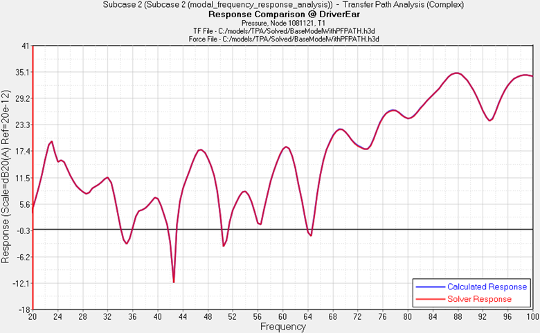
Note: If the option Generate all path contribution plots was checked ON, plots are also generated for:
- The contribution from each dof of the attachment points towards the Calculated Response.
- Transfer Function (TF) for each dof
- Input Force through each dof
- Point Mobility (if requested) for each dof
Figure 8. Path Contribution of dof R1 (Rotation around X) . of One of the Attachment Points Towards the Calculated Response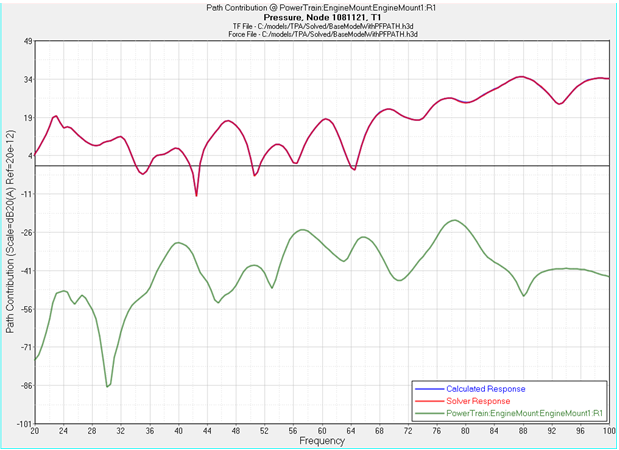

Figure 9. Transfer Function (TF) of dof R1 (Rotation around X) . of One of the Attachment Points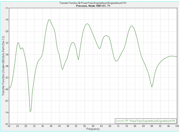

Figure 10. Input Force through dof R1 (Rotation around X) . of One of the Attachment Points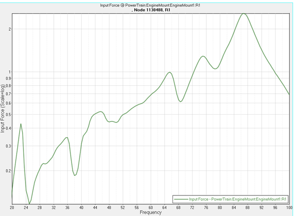

Figure 11. Point Mobility at dof R1 (Rotation around X) . of One of the Attachment Points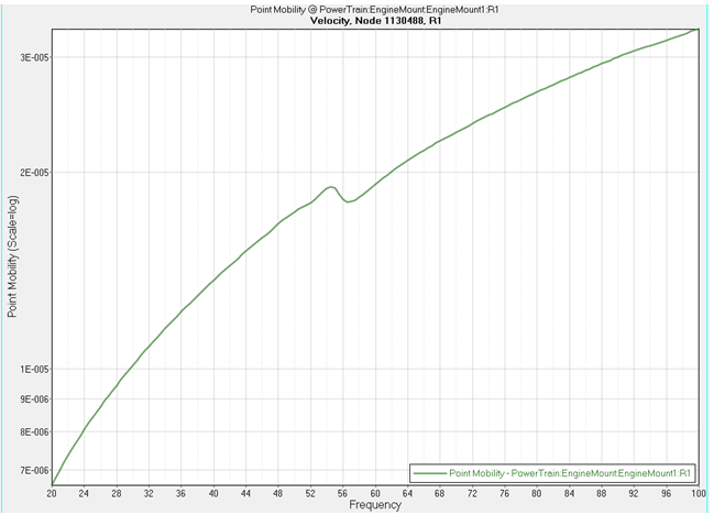
The TPA utility automatically advances to the Display tab. Select the problem frequency, that is, peak in the response which may be over the target level and find the top contributors to the response at that particular frequency.

Note: There are many visualization options available to display the top contributors: Bar Plot (default), Polar Plot, 2D Line, 3D Bar, 3D Surface and Force Vector.
Bar Plot, Polar Plot and Force Vector show the top contributors at a specific frequency; while 2D Line, 3D Bar and 3D Surface show the top contributor over a frequency range.

Shown below are the top contributors at a particular frequency (for example: in this case 47.0 Hz) in Bar Chart format. In the Bar Chart the leftmost bar is for the Response. The contributions are shown in percentage. For the example shown in Figure 12, the top contribution is coming from Engine Mount 3 Y (T3) direction at 55.47%, followed by Engine Mount 2 X (T1) direction at 35.83% etc.

Figure 12. Top Contributors at a Particular Frequency in Bar Plot Format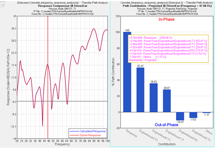

Tip: If the interest is to find the top contributors over a frequency range, then you can use 2D Line, 3D Bar or 3D Surface visualization option.

Attention: Shown below are the top contributors for the frequency range 40.0 Hz to 80.0 Hz using the 2D Line plot. The RSS method is chosen to determine the ranking. The Blue curve in the plot on the RHS is the Total Response. The top contributor over the frequency range 40.0 Hz to 80.0 Hz is Engine Mount 3 Z(T3) direction, followed by Engine Mount 2 Z(T3) direction. You can find more details about other visualization options at Altair HyperWorks > HyperGraph 2D > Graphical User Interface > HyperGraph 2D Menus > NVH Menu > Transfer Path Analysis Utility.

Figure 13. Top Contributors Over a Frequency Range 40.0 Hz to 80.0 Hz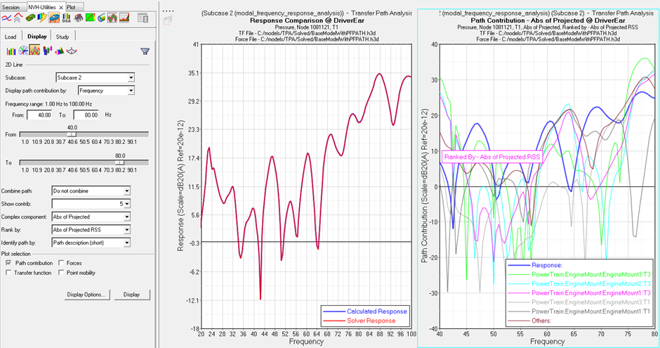
Once the dominant path for a particular problem frequency has been identified, you can use the Study tab to see how much improvement can be made in getting the response down at the problem frequency by excluding the contribution from the dominant paths.
For example: Figure 14 shows how Total Response would change if the top contributing path for 40.0 Hz to 80.0 Hz which is Engine Mount 3 Y(T3) Direction is reduced by 50%.

Figure 14. Effect of Reducing Contribution from Top Contributing Paths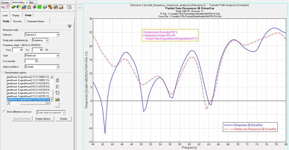

CAUTION:
These results should be interpreted with caution, since this change in response is based on mathematically reducing the contribution of particular paths but when changes are made to the structure to reduce the contribution of certain paths, the structure change changes the modes of the structure, which will then change the response of the structure for the same loading. Nonetheless the Study can be used as to how much potential benefit exists on working on a certain path, before actually investing time in changing the model and running it.