
Co-simulation Introduction
Co-simulation is a simulation methodology that allows complex systems comprised of subsystems to be easily simulated.
How is this is accomplished? Each of the subsystems is simulated in a different simulation tool, but they are executed simultaneously. Relevant signals between them are exchanged during execution at regular intervals and the combined simulation is synchronized so that an orderly exchange of signals is made possible. In the time between the two communication points, the subsystems are solved independently from each other by their individual solvers.
Benefits of Co-simulation
Modeling complex heterogeneous systems in engineering usually leads to hybrid systems. Often, these multi-disciplinary systems cannot be modeled and simulated in one simulation tool alone. Instead, the system needs to be broken up into domain specific subsystem. A co-simulation approach allows organizations to choose the most appropriate simulation tools for each sub-system. By coupling the tools and co-simulating them together, engineers can create and simulate complex hybrid systems.
Applications of Co-simulation
Co-simulation is a potential solution whenever multiple-physics are to be coupled. The following examples, taken from the automotive domain, provide a glimpse of the generality of co-simulation and variety of system-level simulations that can be performed with co-simulation. Similar examples can be found in other industries also.
Vehicle - Controls Interaction
In this scenario, the objective is to understand how well control systems can regulate/control the behavior of a mechanical system. The mechanical system could be a car and the control system could be a steering control system. The vehicle model is defined in MotionSolve and the steering control is defined in a controls package like Altair Twin Activate. The vehicle sends information like vehicle heading and tire slip angles to the controller. The controller computes a steering wheel angle or torque based on these inputs and returns it to the vehicle model.

In this scenario, the objective is to understand how well the hydraulics in a system can regulate/control the behavior of a mechanical system. The mechanical system could be a car and the hydraulic system could be a brake system. The vehicle model is defined in MotionSolve and the steering control is defined in a hydraulics package like DSHPlus (www.fluidon.com). The vehicle sends information like wheel speed and steering wheel angle to the controller. The controller/hydraulics system computes a brake demand and torque based on these inputs and returns it to the vehicle model.

Vehicle - Driver Interaction
In this scenario, the objective is to "drive" a full vehicle model with a driver model and understand how the vehicle responds to the driver input. The driver module includes the vehicle's direction, with its speed as input. The driver is required to make the vehicle follow a specified path at a specified velocity and ensure that the vehicle lateral acceleration is below a target limit. The driver specifies as output the throttle value, the brake pressure, the steering angle and the gearshift value. The vehicle is modeled in MotionSolve. The driver, modeled as a hierarchical control system, is contained in a separate driver module.

Vehicle - Road Interaction
Tires play a critical role in vehicle simulations; they are the only portion of the vehicle that is in contact with the road. Tires are very complex entities consisting of rubber, metal, and plastic. Their behavior is influenced by a variety of internal factors such as air pressure and tread, environmental factors such as temperature and road conditions, and driving conditions such as acceleration, braking, and turning.
Tire and tire-terrain interaction is quite complex and specialized; off-the-shelf tire models are available. Co-simulation is used to couple the tire model to the vehicle model. The vehicle tells the tire where it is in space and how fast it is moving. The tire then calculates the tire-terrain interaction force and tells the vehicle the forces and moments acting at the spindle.
Such a coupling can be quite sophisticated as evidenced by the figure below. The truck-trailer system shown below may have as many as 100 tires. Each of these tires is connected to the vehicle model via co-simulation.

Vehicle - Mechatronics Interaction
Complex systems such as cars and planes have many embedded control systems. These systems monitor and control the behavior of the car or plane to avoid catastrophic failures and ensure high performance. The term, Mechatronics, was coined to define such embedded systems. Figure 5 provides a few examples of mechatronic systems relevant to automobiles. In order to assess the behavior of the controlled vehicle, co-simulation between the vehicle model and the various mechatronic subsystems is necessary.

The Co-simulation Process
- Decomposing a complex system into sub-systems, based on the physics describing the subsystems.
- Creating functional models for each subsystem in the individual simulators and making sure that each subsystem performs as intended.
- Creating the "connections" (signals) between the different subsystems. Typically, there is power transfer from one system to another. So, one subsystem typically receives flow information such as velocity, angular velocity, current, volumetric flow rate or entropy flow rate. In return it sends back to the subsystem from which it received the flow information, effort information such as force, moment, voltage, pressure or temperature.
- Choosing the mechanism for inter-process communication (for example, shared memory on a single machine or TCP/IP for network communication).
- Performing the combined simulation.
Implicit to this process is a sampling strategy to sample the connected signal by each solver, which can be accomplished with different approaches.
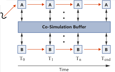
Figure 6 below describes schematically and generally how this may be done between two simulators A and B.
At the sampling times, which may be pre-decided or computed during the co-simulation, each simulator deposits the information it is required to provide to the other simulator into a Co-Simulation Buffer. When Simulator A requires information from B at a certain time, the Co-Simulation Buffer provides this information to A, either by interpolating or extrapolating through data provided by B. Likewise, when Simulator B requires information from A at a certain time, the Co-Simulation Buffer provides this information to B, either by interpolating or extrapolating through data provided to it by A.
Through the use of a co-simulation buffer, many simulators A...N may be coupled. As long each simulator deposits its exchange values at the appropriate frequency, the Simulation Buffer has the ability to provide each simulator with the data it needs from the other simulators.
The MotionSolve implementation of co-simulation using Control_PlantInput, Control_PlantOutput, and FMU statements resembles this process, with a few qualifications to the sampling strategy.
The intent of co-simulation with MotionSolve is to exchange data with another system and use it in a manner that resembles a continuous system. During co-simulation, MotionSolve and the other software (for example, Twin Activate, EDEM, Simulink, and so on) with which it is simulating share data with the Co-Simulation Buffer, as described previously.
The co-simulation is achieved via a leading-lagging approach, where simulator A or B leads the co-simulation, taking the first step, and the other simulator catches up to keep the processes coordinated. Each solver can take whatever time step they choose, but there are some conditions that cause the solver to wait if the data from the other solver is not yet available. The role of MotionSolve as the leading or lagging simulator depends on the type of co-simulation. For example, in a MotionSolve and EDEM co-simulation, MotionSolve is the leading simulator, while in a MotionSolve and Twin Activate co-simulation, MotionSolve takes the role of the lagging simulator.
The data must be coordinated so that the extrapolating solver (the leading solver) is not allowed to take a larger time step than the interpolating solver (the lagging solver), in order to prevent large error from extrapolating too far ahead in time. The interpolating solver cannot take a step if the data is not yet available for the last time step, since by the nature of the interpolation, the data at a future time must be available.