Visualize Results - Animation and Request Plots in MotionSolve
- Easily grasp the physical phenomena.
- Quickly detect errors.
- Create compelling presentations.
 |
 |
 |
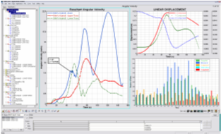 |
These images illustrate the Altair HyperWorks powerful tools for visualizing the results of multibody simulations in the form of 2D and 3D plots and animations.
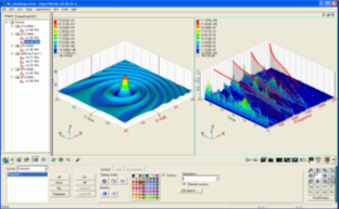
Plots
Plots are essential for obtaining detailed information regarding system behavior as well as for subsequent engineering calculations, such as filtering.
- Altair Binary Format (ABF): This binary file is optimized for fast plotting of very large data sets. This is the recommended format for plotting.
- Multibody Results File (MRF): The primary purpose of this binary file is to provide part displacement data to the post-processor module that creates the H3D file used for animation. The H3D file format is discussed later in this document. The MRF file can also be used to create plots. However, the performance may be slower than the ABF file.
- Plot File (PLT): This is an ASCII file that can be plotted using HyperGraph. The primary purpose of this file is to facilitate load transfers from MotionSolve to FEA software, such as Nastran and OptiStruct, for durability simulation, using the Load Summary utility available in MotionView.
The MRF and ABF files contain, by default, the displacement time histories of all parts and certain other information as shown in the table below:
| Type | Component | Description |
|---|---|---|
| Rigid Body | X, Y, Z | Position |
| E0, E1, E2, E3 | Orientation in Euler parameters. | |
| VM, VX, VY, VZ | Magnitude and X, Y, Z components of velocity. | |
| WM, WX, WY, WZ | Magnitude and X, Y, Z components of angular velocity of the principle inertia axes. | |
| ACCM, ACCX, ACCY, ACCZ | Magnitude and X, Y, Z components of acceleration. | |
| WDTM, WDTX, WDTY, WDTZ | Magnitude and X, Y, Z components of angular acceleration of the principle inertia axes. | |
| Flex Body | X, Y, Z | Position |
| E0, E1, E2, E3 | Orientation in Euler parameters. | |
| Q/i, i = 1, 2, ..., n | Modal participation factors. | |
| QD/i, i = 1, 2, ..., n | Modal velocities. These are written to the output file when the attribute FLEX_VEL_ACC_OUTPUT is set to TRUE in Output: Results | |
| VM, VX, VY, VZ | Magnitude and X, Y, Z components of velocity. These are written to the output file when the attribute FLEX_VEL_ACC_OUTPUT is set to TRUE in Output: Results | |
| QDD/i, i = 1, 2, ..., n | Modal accelerations. These are written to the output file when the attribute FLEX_VEL_ACC_OUTPUT is set to TRUE in Output: Results | |
| ACCM, ACCX, ACCY, ACCZ | Magnitude and X, Y, Z components of acceleration. These are written to the output file when the attribute FLEX_VEL_ACC_OUTPUT is set to TRUE in Output: Results | |
| SE | Strain Energy. | |
| System | KE | Kinetic energy. |
| CPU Usage | Total CPU time used. | |
| CPU/Sim. Time Ratio | The ratio between the total CPU time used and the simulation time. | |
| Stepsize | Actual step size used in the integration. | |
| Integration Order | Order of the integrator used in the integration. |
- Using built-in types for commonly requested data, such as displacement, velocity, and acceleration, as well as forces on bodies and joints.
- Using the MotionSolve expressions. For example, DM(1, 2) returns the distance between the origins of two markers with identifiers 1 and 2.
- Using user-defined subroutines in C/C++, Fortran, or Python.
Refer to the Post: Output Request topic in the XML Format Reference Guide for details.
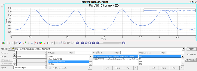
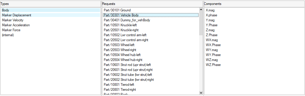
An example of organizing plot data into Type, Request and Component categories.
The following table displays the pre-defined components for each request type.
| Type | Component | Description |
|---|---|---|
| Marker Displacement | DM, DX, DY, DZ | Magnitude and X, Y, Z components of displacement. |
| E0, E1, E2, E3 | Orientation in Euler parameters. | |
| PSI, THETA, PHI or YAW, PITCH, ROLL angles | Orientation of the principle inertia axes expressed in either Euler Angles (B313) or YAW, PITCH, ROLL angles. The choice is made by specifying the ANGLE_TYPE attribute in the Output: Results command. | |
| Marker Velocity | VM, VX, VY, VZ | Magnitude and X, Y, Z components of velocity. |
| WM, WX, WY, WZ | Magnitude and X, Y, Z components of angular velocity of the principle inertia axes. | |
| Marker Acceleration | ACCM, ACCX, ACCY, ACCZ | Magnitude and X, Y, Z components of acceleration. |
| WDTM, WDTX, WDTY, WDTZ | Magnitude and X, Y, Z components of angular acceleration of the principle inertia axes. | |
| Marker Force | FM, FX, FY, FZ | Magnitude and X, Y, Z components of force. |
| TM, TX, TY, TZ | Magnitude and X, Y, Z components of torque. | |
| Expressions | F1, F2, ..., F8 | Vectors containing evaluated expressions. |
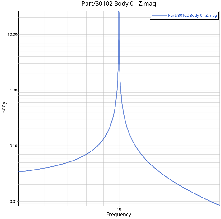
In addition to the above, when you request a linear analysis, MotionSolve writes out a *_linz.mrf file that contains results from the linear analysis. These are described below:
| Type | Component | Description |
|---|---|---|
| Eigenvalue | real part | Real part of the eigenvalue |
| imag part | Imaginary part of the eigenvalue | |
| freq (cycle) | Imaginary part of the
eigenvalue (expressed in cycles per second). freq = (imag part) / 2*PI |
|
| damping ratio | Damping ratio for each eigenvalue | |
| natural freq | Natural frequency for each eigenvalue | |
| Body Eigenvector | dx.real, dy.real, dz.real | Real part of the eigenvector for each body in the system |
| dx.imag, dy.imag, dz.imag | Imaginary part of the eigenvector for each body in the system | |
| % distribution of Kinetic Energy | X, Y, Z | Modal KE distribution in the translational directions for each supported part |
| RXX, RYY, RZZ | Modal KE distribution in the rotational directions for each supported part | |
| RXY, RXZ, RYZ | Modal KE distribution in the cross-rotational directions for each supported part | |
| % distribution of Strain Energy | X, Y, Z | Modal SE distribution in the translational directions for each supported part |
| RX, RY, RZ | Modal SE distribution in the rotational directions for each supported part | |
| % distribution of Dissipative Energy | X, Y, Z | Modal DE distribution in the translational directions for each supported part |
| RX, RY, RZ | Modal DE distribution in the rotational directions for each supported part |
| Type | Component | Description |
|---|---|---|
| Body | X mag, Y mag, Z mag, WX mag, WY mag, WZ mag | Magnitude of frequency response in each direction. |
| X phase, Y phase, Z phase, WX phase, WY phase, WZ phase | Phase of frequency response in each direction. | |
| FlexBody | X mag, Y mag, Z mag, WX mag, WY mag, WZ mag | Magnitude of frequency response in each direction. |
| X phase, Y phase, Z phase, WX phase, WY phase, WZ phase | Phase of frequency response in each direction. | |
| Q/i mag, i = 1, 2, ..., n | Magnitude of frequency response of each mode. | |
| Q/i phase, i = 1, 2, ..., n | Phase of frequency response of each mode. | |
| Marker Displacement | X mag, Y mag, Z mag, WX mag, WY mag, WZ mag | Magnitude of frequency response in each direction. |
| X phase, Y phase, Z phase, WX phase, WY phase, WZ phase | Phase of frequency response in each direction. | |
| Marker Velocity | X mag, Y mag, Z mag, WX mag, WY mag, WZ mag | Magnitude of frequency response in each direction. |
| X phase, Y phase, Z phase, WX phase, WY phase, WZ phase | Phase of frequency response in each direction. | |
| Marker Acceleration | X mag, Y mag, Z mag, WX mag, WY mag, WZ mag | Magnitude of frequency response in each direction. |
| X phase, Y phase, Z phase, WX phase, WY phase, WZ phase | Phase of frequency response in each direction. | |
| Marker Force | X mag, Y mag, Z mag, WX mag, WY mag, WZ mag | Magnitude of frequency response in each direction. |
| X phase, Y phase, Z phase, WX phase, WY phase, WZ phase | Phase of frequency response in each direction. |
Animation
Animations not only provide a quick way to check for errors, they also help create compelling presentations to communicate your results to a wide audience.
MotionSolve creates the following two file types for animation, based on your selected simulation type. The H3D file is used to animate static, quasi-static, linear, and transient simulation results. The H3D file contains both the graphics as well as the results information.
MotionSolve writes the complex nodal displacement to H3D in the _linz.h3d file, HyperView performs modal animation, and you can leverage the features of the NVH Director.
MotionSolve writes the frequency response analysis results to H3D in the _frf.h3d file.
- Compact file size with additional compression options
- Fast animation
- Single format for sharing engineering animation results from finite element as well as multibody dynamics software
- H3D files may be animated using the stand alone HyperView Player
You may use the Post_Graphic modeling element to add graphics to visualize the elements in your models. Below is a summary of the different types of graphics available in MotionSolve. For details, see Post: Graphic in the MotionSolve XML Format Reference Guide.
Rigid Bodies
You can choose from the following types of graphics to visualize rigid bodies:
| ArcFromRadius ArcFromRM BoxDefinedFromCenter |
BoxDefinedFromCorner CircleFromRadius CircleFromRM |
Cylinder Ellipsoid Frustum |
Plane Sphere TriaMesh Parasolid |
Note that these graphics are useful for visualization and contact only. They do not affect the mass and inertia properties. For example, when you use a box graphic to visualize a body, its mass and moments of inertia are not calculated based on the box geometry and material properties.
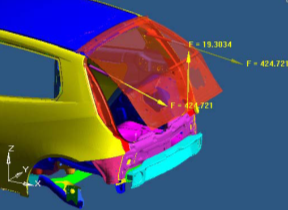
Forces and Moments
Outline
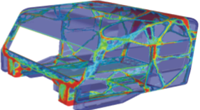
Flexible Bodies
- Contour plots
Figure 6. Result Contours for CMS Flexible Control Arms for a SLA Suspension Model 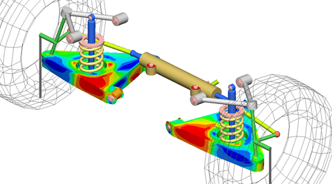
Figure 7. Result Contours for an NLFE Stabilizer Bar in a Front Suspension Model 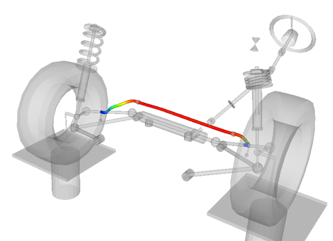
You may contour results of various types including displacements, rotation (CMS only), velocity (CMS only), acceleration (CMS only), strain, and stress. For strain and stress, you must request the corresponding modes to be computed during the component mode synthesis solution for a CMS flexible component; for an NLFE body, these are written to the H3D by default.
Note: The NLFE element results are always written in NODAL format whereas the CMS flexible results can be written in NODAL or MODAL format (this is controlled by the FORMAT_OPTION) attribute in the H3DOutput command statement. - Vector plots
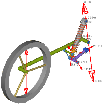
Figure 8. Displacement Vectors for an NLFE Beam Superimposed on the Stress Contour Plot 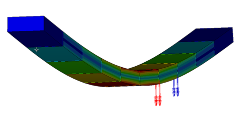
You may create vector plots of the following data types: displacement, velocity (CMS only), acceleration (CMS only), force (CMS only), and moment (torque, CMS only). The vectors may be resolved in a variety of coordinate systems. Scaling and querying are also supported. The vector plots can also be overlaid over the stress contour plots.
- Tensor plots
Figure 9. Stress Tensors for a Control Arm in an SLA Suspension 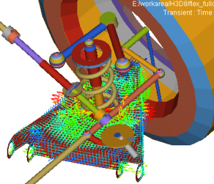
You may create tensor plots to visualize tensor quantities such as stress and strain. Two formats are available - Principal or Component. The tensors may be resolved in a variety of coordinates systems. Nodal averaging is also supported.
For all these visualization approaches, displacements and deformations are available by default, while stresses and strains must be requested during the component mode synthesis (CMS) solution.
For the NLFE bodies, displacements, stresses and strain information is written by default to the H3D.
3D Rigid Body Contact
During a simulation that contains rigid body contact elements, MotionSolve computes a number of contact related quantities like normal force, friction force, slip velocities etc. These are written to the H3D after the simulation so that they can be visualized in HyperView.
- Contact summary frame:The contact summary frame is a single frame in HyperView which allows you to visualize the maximum penetrations that occurred in your 3D geometries over the length of the entire simulation. A sample contact summary frame is shown below (in exploded view).
Figure 10. Contact Summary Frame for Bevel Gears in Contact 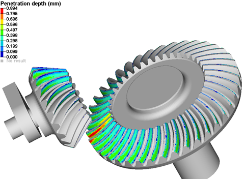
MotionSolve writes an additional load case, called “Contact Overview” to the animation H3D file when the model contains active 3D rigid body contact(s). Within this load case, you can create a contour plot defined by maximum penetration depth.
The summary frame allows you to quickly check for excessive penetrations in your simulation before animating it. It can also be used to assess whether the areas where contact occurred are as expected. For more information on the contact summary frame, please see the Post-processing section in 3D Mesh-to-Mesh Contact Simulation.
- Vector plots:You may also use vector plots to display contact forces and velocities. In addition to the total contact force, you can visualize several other results including contact friction force:
Figure 11. Contact Related Vector Plot Results 
Figure 12. Normal Contact Force for a Constant Velocity Joint Geometry 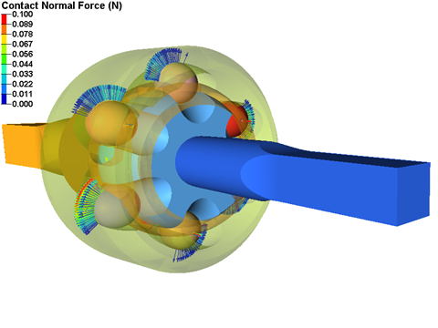
You can plot these vectors for each triangular element on the rigid body or for a contact region.
- Contour plots:You may also use vector plots to display contact forces and velocities. In addition to the total contact force, you can visualize several other results including contact friction force:
- Contact force (including normal and friction force)
- Contact velocity (including normal and tangential velocities)
- Contact penetration depth
Figure 13. Total Contact Force Contour for a Constant Velocity Joint Geometry 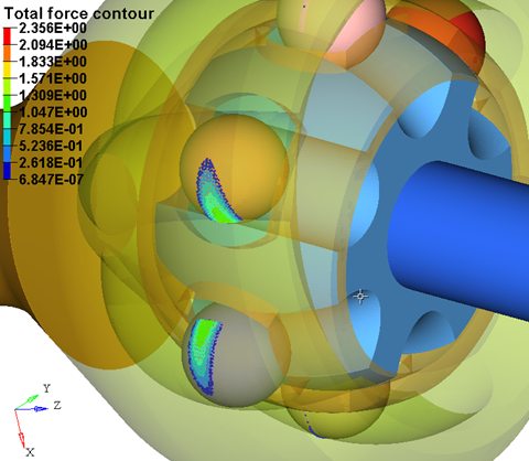
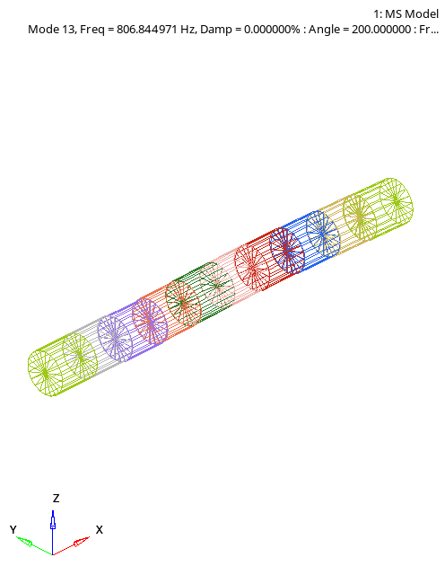
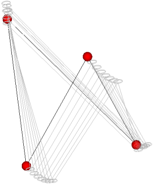
Linear Modes
- MotionSolve computes and writes the displacements for each mode as transient results from 0 to 360 degrees from complex results in the *..h3d file.
- MotionSolve writes the complex nodal
displacement to H3D in the
_linz.h3d file, and HyperView performs the modal animation.
Figure 14. Linear results from H3D results 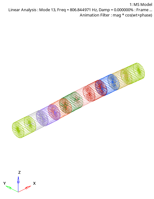
Figure 15. Linear results from Linz H3D