HS-4425: Multi-Objective Shape Optimization Study
Perform a multi-objective Optimization study, and search for the Pareto front that minimizes both volume and maximum displacement.
Run Multi-Objective Shape Optimization
-
Add an Optimization.
- In the Explorer, right-click and select Add from the context menu.
- In the Add dialog, select Optimization.
- For Definition from, select Setup and click OK.
-
Modify input variables.
- Go to the step.
- In the work area, Active column, clear the radius_1, radius_2 and radius_3 checkboxes.
- Go to the step.
- Click the Objectives/Constraints - Goals tab.
-
Apply an objective on the Volume and Max_Disp output responses.
Figure 1. 
-
Click the Define Output Responses step, and change the
Evaluate From column to Fit - RBF (fit_4) for Volume,
Max_Stress, and Max_Disp.
Figure 2. 
- Go to the step.
- In the work area, set the Mode to Multi_Objective Genetic Algorithm (MOGA).
- Click Apply.
- Go to the step.
-
Click Evaluate Tasks.
HyperStudy stops MOGA after 50 iterations, and performs a total of 13317 analyses. The Pareto front of the last iteration contains 408 points.
- Go to the step.
-
Click the Optima tab.
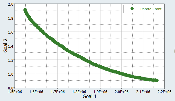
The Pareto front of Objective 2 versus Objective 1 is displayed in the plot.
The goal of this study was to minimize both Volume (Objective 1) and Max_Disp (Objective 2). The Pareto plot shows all of the non-dominated solutions. A non-dominated solution is a solution which can no longer improve one objective without deteriorating another. You can see that minimizing Objective 1 will increase Objective 2, and minimizing Objective 2 will increase Objective 1. According to these results, you must decide what would be the optimal solution. For instance, the Pareto plot may allow a compromise solution to be selected somewhere in the middle.
Figure 3.