
ACU-T: 3600 Melting of Diesel Exhaust Additive within an Enclosed Tank
Tutorial Level: Advanced
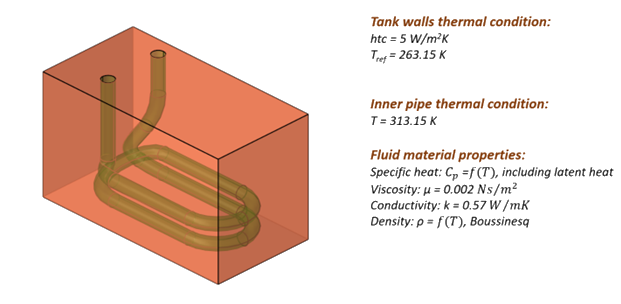
This tutorial provides the directions for setting up, solving, and post-processing results for a simulation that models the approximated melting of the common diesel fuel exhaust additive that is contained within a notional tank. Prior to starting this tutorial, you should have already run through the introductory tutorial, ACU-T: 1000 Basic Flow Set Up, and have a basic understanding of HyperMesh CFD and AcuSolve. To run this simulation, you will need access to a licensed version of HyperMesh CFD and AcuSolve.
Problem Description
Start HyperMesh CFD and Open the HyperMesh Database
- Start HyperMesh CFD from the Windows Start menu by clicking .
-
From the Home tools, Files tool group, click the Open Model tool.
Figure 2. 
The Open File dialog opens. - Browse to the directory where you saved the model file. Select the HyperMesh file ACU-T3600_UreaTankMelting_TemperatureBasedEffectiveness.hm and click Open.
- Click .
-
Create a new directory named MeltingTank and navigate into this directory.
This will be the working directory and all the files related to the simulation will be stored in this location.
- Enter MeltingTank as the file name for the database, or choose any name of your preference.
- Click Save to create the database.
Validate the Geometry
The Validate tool scans through the entire model, performs checks on the surfaces and solids, and flags any defects in the geometry, such as free edges, closed shells, intersections, duplicates, and slivers.
Set Up Flow
Set Up the Simulation Parameters and Solver Settings
-
From the Flow ribbon, click the Physics tool.
Figure 4. 
The Setup dialog opens. -
Under the Physics models setting:
-
Click
 beside the time step field and select
Modify time integration settings. Set the
Time integration order to First.
beside the time step field and select
Modify time integration settings. Set the
Time integration order to First.
Figure 5. 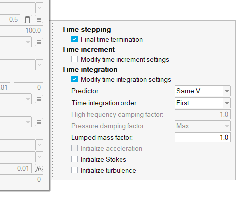
Figure 6. 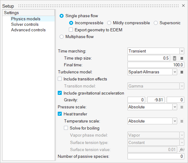
-
Click
-
Under the Advanced controls setting, set the minimum stagger iterations to
1 and the maximum to 4.
Figure 7. 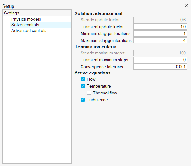
Assign Material Properties
-
From the Flow ribbon, click the Material Library tool.
Figure 8. 
- Under Settings, click Fluid, and then click the My Materials tab.
-
Click
 to create a new material.
-
Name the material Urea, set the density (ρ) type to
Boussinesq and enter Density (kg/m3) and
Reference temperature (K) values as shown below.
Figure 9. 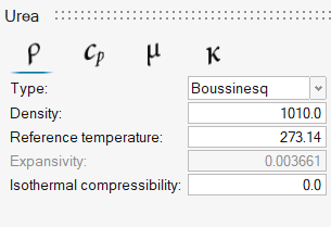
- Click the Specific Heat tab and set the Type to Piecewise Linear Enthalpy.
- Verify that the Curve fit variable is set to Temperature.
- Set the Latent heat type to Constant.
- Enter the values for Latent heat (J), Latent heat temperature (K), and Latent heat temperature interval (K) by referring to the figure below.
-
Click
 three times to add three rows to the table and then
enter the table values according to the figure below.
three times to add three rows to the table and then
enter the table values according to the figure below.
Figure 10. 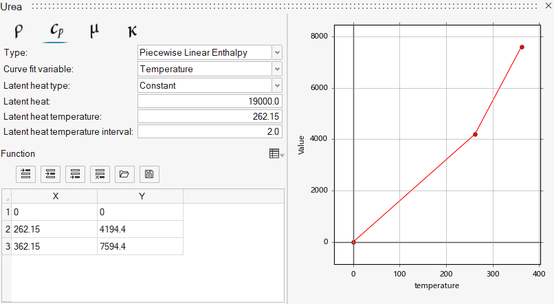
- Click the Viscosity tab and set µ (viscosity) to 0.002 kg/m-sec.
- Click the Conductivity tab and set k (conductivity) to 0.57 W/m-K.
- Close the material creation dialog.
-
From the Flow ribbon, click the Material tool.
Figure 11. 
-
Assign the Fluid material – Urea – to the tank volume, as shown in the figure
below.
Figure 12. 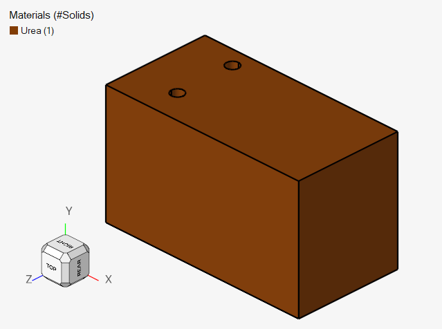
Define the Porous Medium
-
From the Flow ribbon, Porous
tool group, click the Cartesian Porous Media tool.
Figure 13. 
- Select the tank volume (urea fluid body).
-
Click Orientation on the guide bar and then choose an arbitrary location to define the Porous model
orientation.
Any location is acceptable for this model.
-
Assign the Porous Media values according to the following figure.
Figure 14. 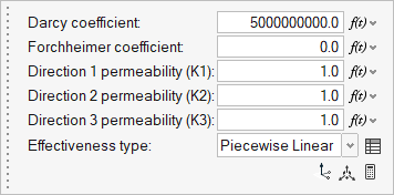
-
Click
 besides Effectiveness type.
-
In the new dialog, click four time to add four empty rows to the table then
enter values according to the figure below.
Figure 15. 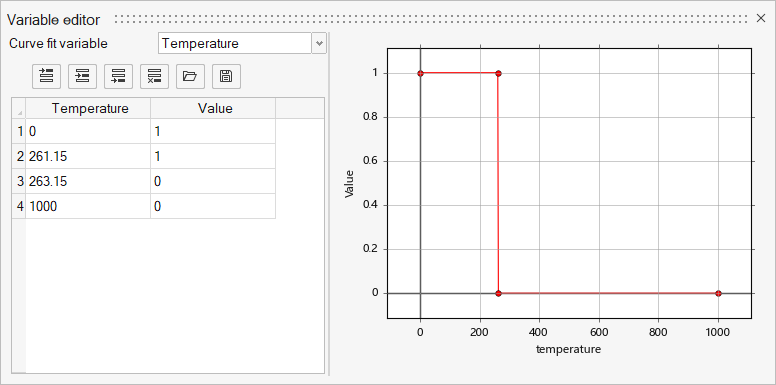
-
Rename the Porous model.
- Double-click Porous in the legend on the left side of the modeling window.
- Type Additive and press Enter.
-
On the guide bar, click
 to execute
the command and exit the tool.
to execute
the command and exit the tool.
Assign the Flow Boundary Conditions
-
From the Flow ribbon, click the No Slip tool.
Figure 16. 
-
Select the exterior faces of the plastic tank.
Figure 17. 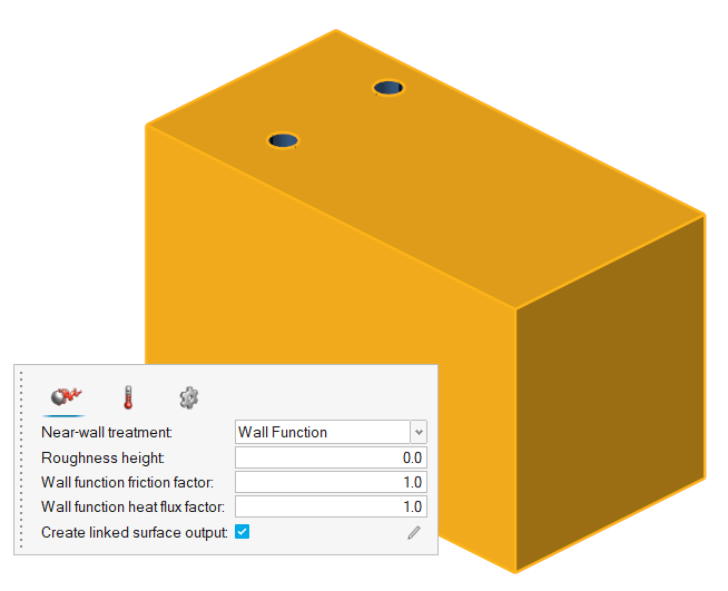
- In the microdialog, click the Temperature tab.
- Verify that the Thermal boundary condition is set to Flux.
- Set the Convective heat coefficient to 5.0 W/m2K.
-
Set the Convective heat reference temperature to 263.15
K.
Figure 18. 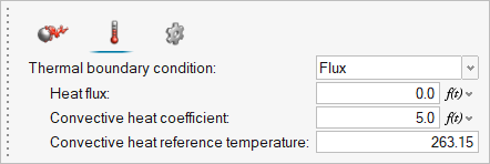
-
Rename the wall boundary.
- Double-click Wall in the legend on the left side of the modeling window.
- Type Exterior_Wall and press Enter.
-
On the guide bar, click
 to execute the command and remain in the
tool.
to execute the command and remain in the
tool.
- Hide Exterior_Wall and select the interior faces of the heating element.
- In the microdialog, click the Temperature tab.
-
Change the Thermal boundary condition to Temperature and
set the Temperature (K) to 313.15.
Figure 19. 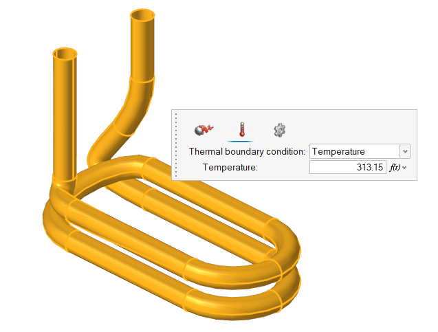
- Double-click Wall in the legend and rename it to Pipe.
-
Click
 on the guide bar.
Generate the Mesh
-
From the Mesh ribbon, click the
Volume tool.
Figure 20. 
-
Set the Maximum element size (m) to 0.02 and verify the
geometric feature angle (degree) is set to 12.5.
Figure 21. 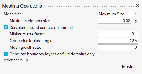
-
Click Mesh.
The Run Status dialog opens. Once the run is complete, the status is updated and you can close the dialog.Tip: Right-click the mesh job and select View log file to view a summary of the meshing process.
Set the Field Outputs
-
Form the Solution ribbon, click the Field tool.
Figure 22. 
- Uncheck Write results at time step interval.
- Check Write results at time interval.
-
Set the Time interval to 1 sec.
Figure 23. 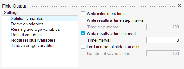
Run AcuSolve
-
From the Solution ribbon, click the Run tool.
Figure 24. 
The Launch AcuSolve dialog opens. - Set the Parallel processing option to Intel MPI.
- Optional: Set the number of processors to 4 or 8 based on availability.
-
Set the Default initial conditions as in the following figure.
Figure 25. 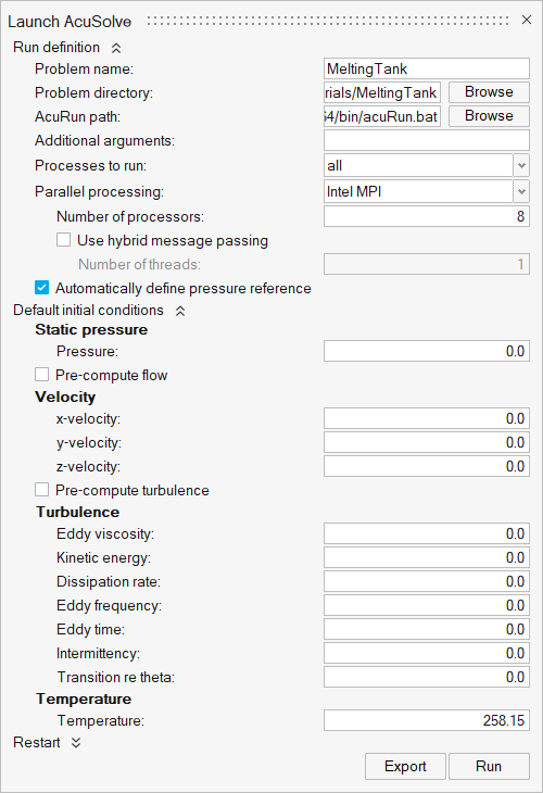
- Leave the remaining default options and then click Run to launch AcuSolve.
Post-Process the Results
Post-Process with the Plot Tool
-
From the Solution ribbon, click the Manage tool.
Figure 26. 
-
In the Run Status dialog, right-click the AcuSolve run and select Plot time
history to launch the Plot Manager.
The residual and solution ratios for pressure, velocity, eddy viscosity, and temperature are shown.
Figure 27. 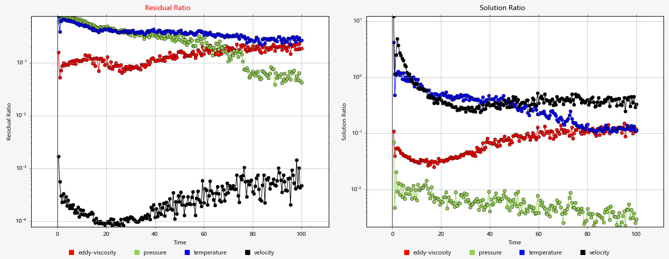
-
Click to define a new plot.
- Expand and select heat flux.
-
Select Pipe – Output to plot the heat flux entering the
domain from the heating element.
Note: The value stabilizes near the end of the simulation, indicating that the model is approaching the prescribed thermal boundary conditions.
Figure 28. Integrated heat flux entering the domain from the heating element surface 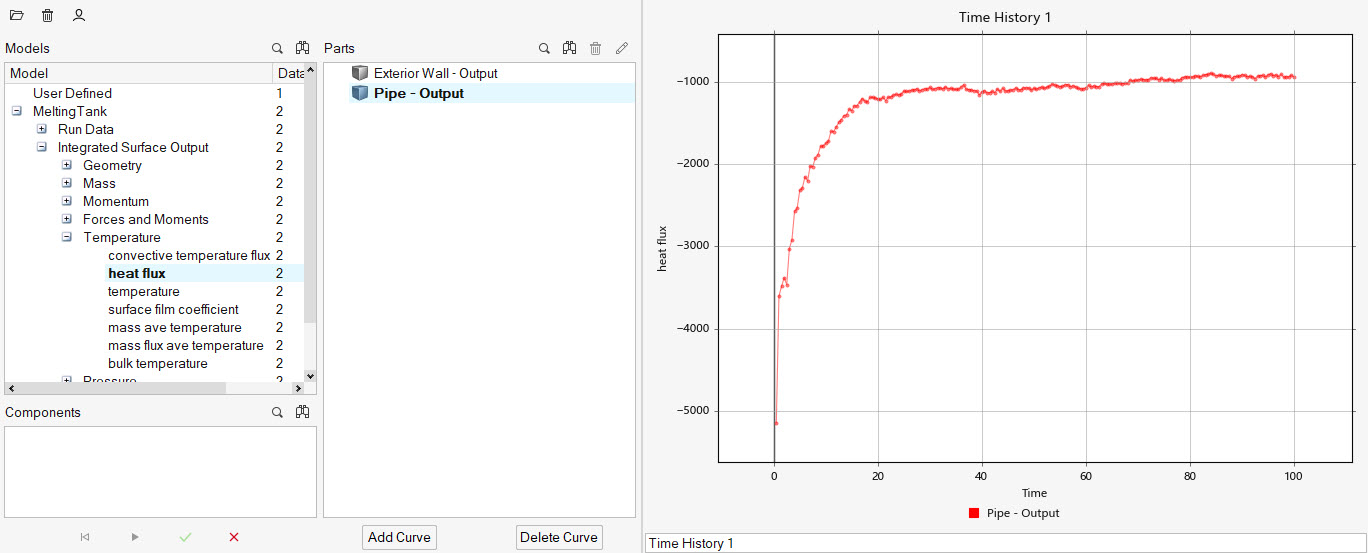
- Expand the .
-
Select the Exterior Wall – Output to plot the
temperature increase of the inside wall of the tank.
Note: The value is not stabilized by the end of the simulation, indicating that the model has not reached the final temperature to balance the prescribed thermal boundary conditions.
Figure 29. Integrated temperature on the interior surface of the tank wall 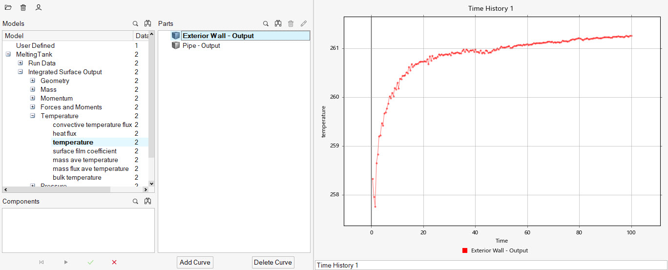
Post-Process with HyperMesh CFD Post
- In the Run Status dialog, right-click the AcuSolve run and select Visualize results to launch HyperMesh CFD Post.
-
From the Post ribbon, click the Boundary Groups
tool.
Figure 30. 
-
Click
 on the guide bar to open the
Advanced Selection dialog.
on the guide bar to open the
Advanced Selection dialog.
-
Select Exterior_Wall - Output and then close the
dialog.
Figure 31. 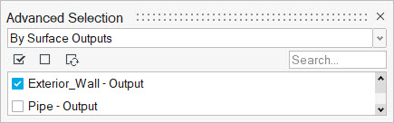
- Set the transparency of the Boundary Group to approximately 75%.
-
On the guide bar, click
to execute
the command and exit the tool.
-
From the Post ribbon, click the Iso-Surfaces tool.
Figure 32. 
-
Select temperature as the Iso Variable and set the Iso
Value of temperature (K) to 261.15.
Figure 33. 
- Click Calculate.
-
In the display properties microdialog, define the
Display as constant and select a color of choice.
Figure 34. Transparent boundary of the tank, showing an Iso-Surface of temperature T=261.15 K, Time=0.0 sec 
-
Using the results animation toolbar, skip to the end of the simulation
results.
Figure 35. Transparent boundary of the tank, showing an Iso-Surface of temperature T=261.15 K, Time=100.0 sec 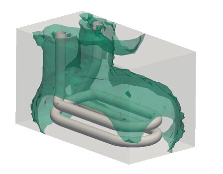
Summary
In this tutorial, you learned how to set up and solve a flow and thermal simulation with temperature dependent porous media effectiveness. Utilizing the proposed implementation allowed you to specify the melting point of a fluid and compute the melted region of the fluid. You started by importing the HyperMesh CFD input database and then you defined the porous medium to control the melting point of the fluid. Next, you assigned the thermal boundary conditions and generated the mesh. Once the solution was computed, you created a plot of the heat flux and temperature for the critical surfaces with the model using HyperMesh CFD Plot Manager.