
ACU-T: 3300 Modeling of a Heat Exchanger Component
Tutorial Level: Beginner
This tutorial provides instructions for modeling a heat exchanger component using HyperMesh CFD. Prior to starting this tutorial, you should have already run through the introductory tutorial, ACU-T: 1000 Basic Flow Set Up, and have a basic understanding of HyperMesh CFD and AcuSolve. To run this simulation, you will need access to a licensed version of HyperMesh CFD and AcuSolve.
Problem Description
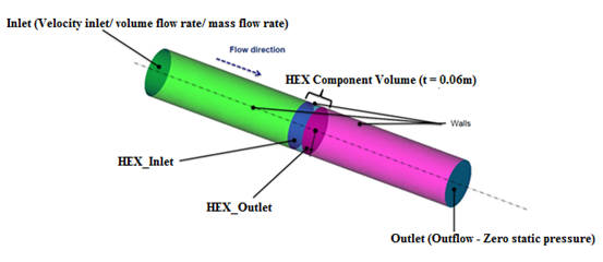
Heat exchangers are devices used to facilitate heat exchange between two fluids that are at different temperatures. A typical heat exchanger device has two separate flows, the cross flow and tubular flow. Depending on the temperatures, heat can flow to or from one fluid to the other through the solids separating them. Since the heat exchanger geometry is quite complex with a large number of plates and pipes, it is not realistic to model the actual heat exchanger when performing system level simulations. In such scenarios, a simplified approach can be employed where only the effect of the heat exchanger on the cross flow is considered instead of modeling the actual heat exchanger. This is done using the heat exchanger component available in AcuSolve.
The heat exchanger component has two effects on the cross flow:
- Pressure drop which is calculated based on the friction parameters provided by the user.
- Heat addition or removal based on the coolant heat transfer parameters.
Start HyperMesh CFD and Open the HyperMesh Database
- Start HyperMesh CFD from the Windows Start menu by clicking .
-
From the Home tools, Files tool group, click the Open Model tool.
Figure 2. 
The Open File dialog opens. - Browse to the directory where you saved the model file. Select the HyperMesh file ACU-T3300_HeatExchanger.hm and click Open.
- Click .
-
Create a new directory named HeatExchanger and navigate into this directory.
This will be the working directory and all the files related to the simulation will be stored in this location.
- Enter HeatExchanger as the file name for the database, or choose any name of your preference.
- Click Save to create the database.
Validate the Geometry
The Validate tool scans through the entire model, performs checks on the surfaces and solids, and flags any defects in the geometry, such as free edges, closed shells, intersections, duplicates, and slivers.
Set Up Flow
Set the General Simulation Parameters
-
From the Flow ribbon, click the Physics tool.
Figure 4. 
The Setup dialog opens. -
Under the Physics models setting:
- Verify that Time marching is set to Steady.
- Select Spalart-Allmaras as the Turbulence model.
- Activate the Heat transfer checkbox.
Figure 5. 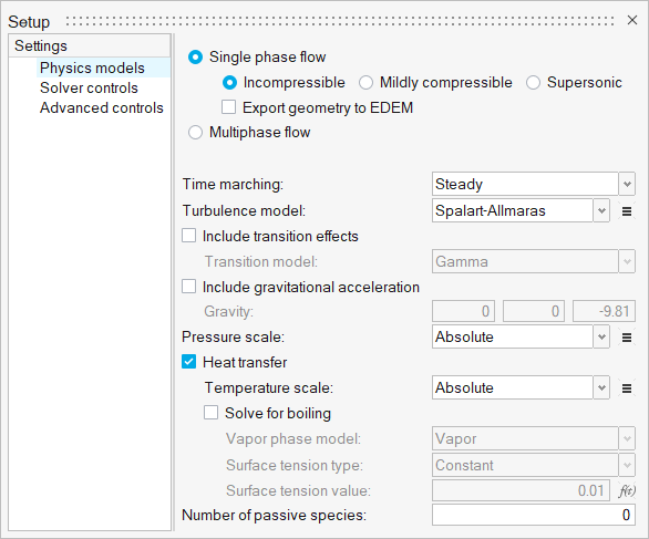
- Close the dialog and save the model.
Assign Material Properties
-
From the Flow ribbon, click the Material tool.
Figure 6. 
- Verify that the Air material has been assigned to all three volumes.
-
Click
 on the guide bar to exit the tool.
Define the Heat Exchanger Component
-
From the Flow ribbon, click the arrow next to the
Domain tool set, and then select
Heat Exchanger.
Figure 7. 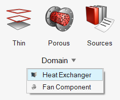
-
Select the middle solid as the heat exchanger component volume.
Figure 8. 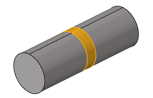
-
On the guide bar, click Inlet and
then select the face shown below as the inlet of the heat exchanger
component.
Figure 9. 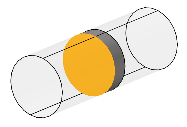
-
In the microdialog, enter the following
parameters:
Figure 10. 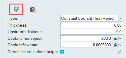
Figure 11. 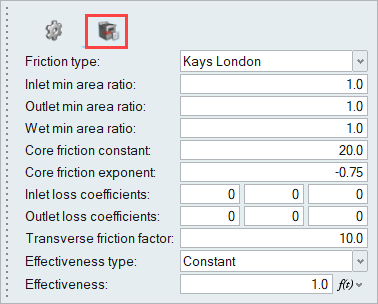
-
On the guide bar, click
 to execute
the command and exit the tool.
to execute
the command and exit the tool.
- Save the model.
Define Flow Boundary Conditions
-
From the Flow ribbon, click the Constant tool.
Figure 12. 
-
Click the inlet face highlighted in the figure below.
Figure 13. 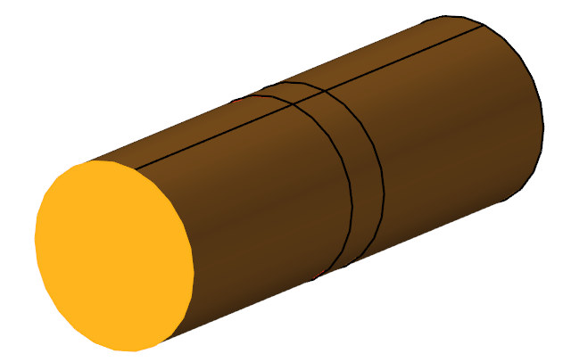
-
In the microdialog, enter the following values for the
Momentum and Turbulence tabs.
Figure 14. 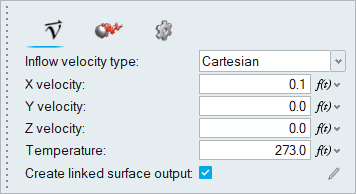
Figure 15. 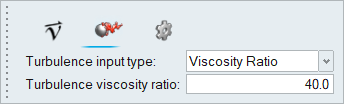
-
On the guide bar, click
to execute
the command and exit the tool.
-
Click the Outlet tool.
Figure 16. 
-
Select the face highlighted in the figure below and then click on the
guide bar.
Figure 17. 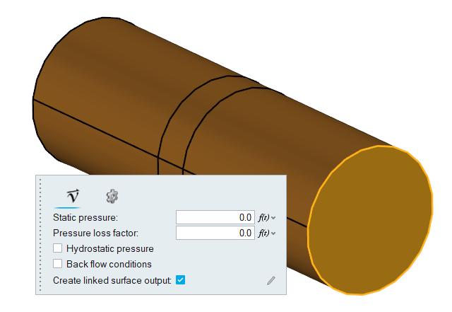
- Save the model.
Generate the Mesh
-
From the Mesh ribbon, click the
Volume tool.
Figure 18. 
-
In the Meshing Operations dialog, set the Mesh growth rate
to 1.1 (if not set already).
Figure 19. 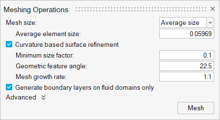
-
Click Mesh.
The Run Status dialog opens. Once the run is complete, the status is updated and you can close the dialog.Tip: Right-click the mesh job and select View log file to view a summary of the meshing process.
- Save the model.
Run AcuSolve
-
From the Solution ribbon, click the Run tool.
Figure 20. 
The Launch AcuSolve dialog opens. - Set the Parallel processing option to Intel MPI.
- Optional: Set the number of processors to 4 or 8 based on availability.
-
Leave the remaining options as default and click
Run to launch AcuSolve.
Figure 21. 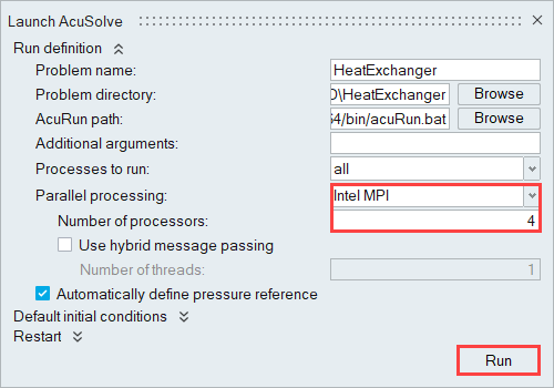
Post-Process with the Plot Tool
-
In the Run Status dialog, right-click the AcuSolve run.
Figure 22. 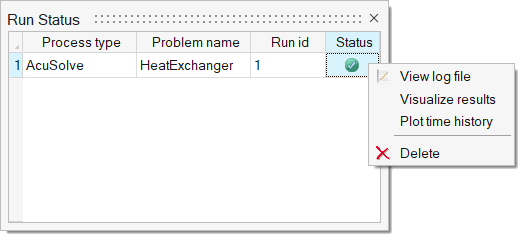
-
Select Plot time history to plot the residual and
solution ratios.
Figure 23. 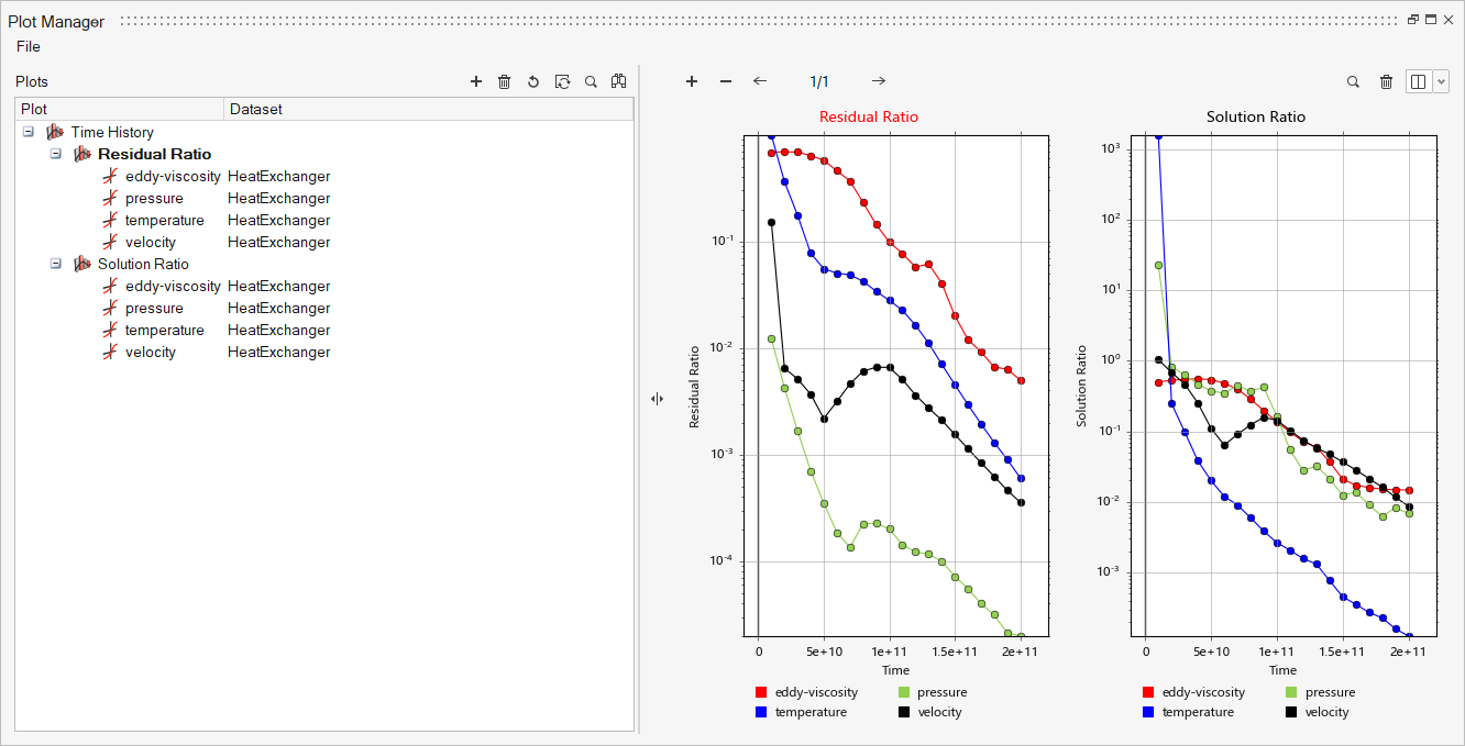
-
Click
 to create a new plot.
- Right-click User Defined under the Model panel to create a user defined function.
- In the Data Tree, expand Heat Exchanger Component Output and then select coolant temperature.
- In the Name field, enter dT.
- In the Value field, type value=.
-
Under Parts, choose HX component and then click
 to insert the field as part of the value, as shown
below.
to insert the field as part of the value, as shown
below.
Figure 24. 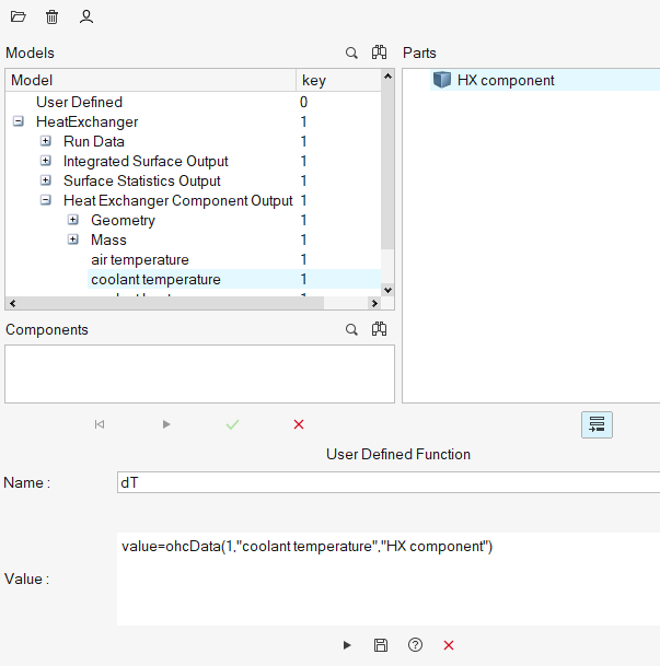
- Type - at the end of the user defined function value.
-
In the Data Tree, select air temperature, and then pick
HX component and click to insert the field as part of the value.
-
Click
 to add the user defined function.
Figure 25. 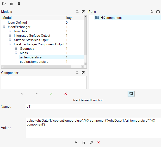
-
Click the x axis to switch to Time Steps.
Figure 26. 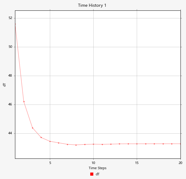
As shown in the plot above, the temperature rise is 43.3K.
Summary
In this tutorial, you successfully learned how to set up and solve a simulation involving a Heat Exchanger component using HyperMesh CFD. You started by opening the HyperMesh input file with the geometry and then defined the simulation parameters, the heat exchanger component, and the flow boundary conditions. Once the solution was computed, you defined a user-function in the Plot Manager in order to create a plot of the temperature rise across the heat exchanger volume.