
ACU-T: 1000 Basic Flow Set Up
Tutorial Level: Beginner
This tutorial introduces you to the workflow for setting up a Computational Fluid Dynamics (CFD) analysis using Altair HyperMesh CFD. HyperMesh CFD is a powerful tool which provides a single, streamlined platform for performing a CFD analysis, starting from importing CAD through post-processing results. In this tutorial, you will learn how to use HyperMesh CFD for setting up a CFD analysis while exploring different capabilities available within the software for importing a geometric model, validating the geometry, setting up simulation parameters and boundary conditions, and generating a mesh. You will then launch AcuSolve simulation directly from HyperMesh CFD and post-process the results using HyperMesh CFD Post.
Prerequisites
To run this simulation, you will need access to a licensed version of HyperMesh CFD and AcuSolve.
Analyze the Problem
An important step in any CFD simulation is to examine the engineering problem at hand and determine the important parameters that need to be provided to AcuSolve. Parameters can be based on geometrical elements, such as inlets, outlets, or walls, and on flow conditions, such as fluid properties, velocity, or whether the flow should be modeled as turbulent or as laminar.

Start HyperMesh CFD and Create the HyperMesh Model Database
-
Start HyperMesh CFD from the Windows Start
menu by clicking .
When HyperMesh CFD is loaded, the Geometry ribbon is open by default.
-
Create a new .hm database in
one of the following ways:
- From the menu bar, click .
Figure 2. 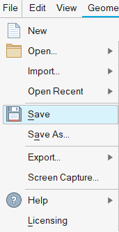
- From the Home tools, Files tool group, click the Save As tool.
Figure 3. 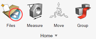
- From the menu bar, click .
-
In the Save File As dialog, navigate to the directory
where you would like to save the database.
This will be your problem directory and all the files related to the simulation will be stored in this location.
- Enter a name for the database (Manifold, for example) and then click Save.
Import and Validate the Geometry
Import the Geometry
- From the menu bar, click .
- In the Import File dialog, browse to your working directory and then select ACU-T1000_manifold.x_t and click Open.
-
In the Geometry Import Options dialog, leave all the
default options unchanged and then click Import.
Figure 4. 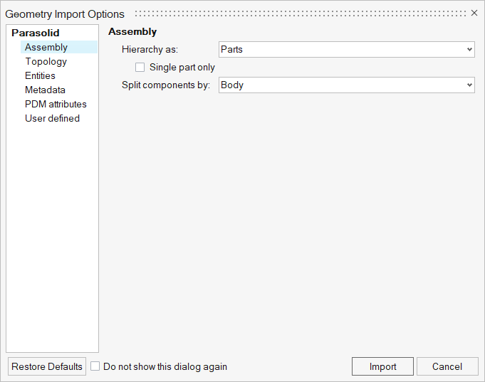
-
Once the geometry is loaded, rotate and observe the features of the model.
The view of the model displayed in the modeling window can be controlled using the following view controls.
Button View Control Middle mouse scroll Zoom in and out Right-click hold and drag Pan the model Middle mouse click hold and drag Rotate the model Figure 5. 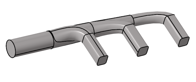
Validate the Geometry
-
From the Geometry ribbon, click the Validate tool.
Figure 6. 
The Validate tool scans through the entire model, performs checks on the surfaces and solids, and flags any defects in the geometry, such as free edges, closed shells, intersections, duplicates, and slivers.The current model does not have any of the issues mentioned above. Alternatively, if any issues are found, they are indicated by the number in the brackets adjacent to the tool name.
Observe that a blue check mark appears on the top-left corner of the Validate icon. This indicates that the tool found no issues with the geometry model.Figure 7. 
- Press Esc or right-click in the modeling window and swipe the cursor over the green check mark from right to left.
- Save the database.
Set Up the Problem
Set Up the Simulation Parameters and Solver Settings
-
From the Flow ribbon, click the Physics tool.
Figure 8. 
The Setup dialog opens. -
Under the Physics models setting:
Figure 9. 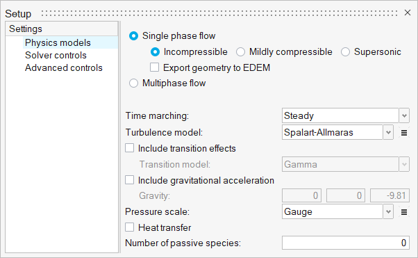
-
Click the Solver controls setting and verify that the
parameters are set as shown in the figure below.
Figure 10. 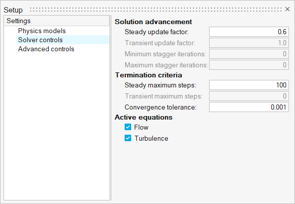
- Close the dialog and save the model.
Assign Material Properties
-
From the Flow ribbon, click the Material tool.
Figure 11. 
-
From the modeling window, click anywhere on the
manifold.
The entire manifold geometry is highlighted and a Material microdialog appears.
Figure 12. 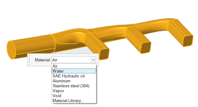
- Click the drop-down menu and select Water from the list of materials.
-
On the guide bar, click
 to execute the command.
The changes made in the tool are not effective until they are executed by clicking the icon.Once the command is executed, the color of the geometry changes to indicate the material assigned to the volume. In this case, there is only one volume in the geometry so there is a single color. Alternatively, if there are multiple volumes with different materials assigned, the model will be displayed accordingly with distinct colors for each material assigned.
to execute the command.
The changes made in the tool are not effective until they are executed by clicking the icon.Once the command is executed, the color of the geometry changes to indicate the material assigned to the volume. In this case, there is only one volume in the geometry so there is a single color. Alternatively, if there are multiple volumes with different materials assigned, the model will be displayed accordingly with distinct colors for each material assigned.Figure 13. 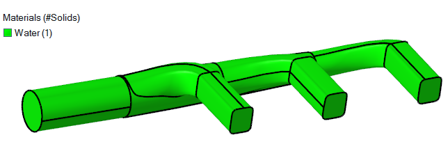
-
On the guide bar, click
 to exit the
tool.
to exit the
tool.
Assign the Flow Boundary Conditions
The current model has one inlet, three outlets, and walls for the rest of the surfaces. When a geometry model is imported into HyperMesh CFD, all the surfaces are placed in the Default Wall (i.e. Type = auto_wall). As you start assigning the surface boundary conditions, those surfaces are moved into a new boundary condition group. All the surface boundary condition tools are placed under the Boundaries sub-section of the Flow ribbon.
-
From the Flow ribbon, Profiled
tool group, click the Profiled Inlet tool.
Figure 14. 
-
In the modeling window, click the surface of the
inlet.
Figure 15. 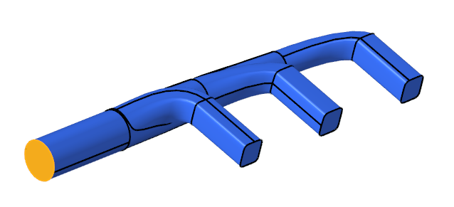
Observe that a new group named "Inlet" is created under the Boundaries list in the top-left corner of the modeling window. Once the current command is executed, the highlighted surface will be moved into the Inlet group. -
In the microdialog, enter a value of
2.0 m/sec for Average velocity.
Figure 16. 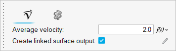
-
On the guide bar, click
to execute the command.
The color of the inlet surface in the modeling window is updated.Note: The color assigned to the surfaces is random. Therefore, the color of the surfaces shown in the images below might be different from what you see on your screen.
Figure 17. 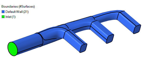
-
Click the Outlet tool.
Figure 18. 
-
Click the three outlet surfaces shown in the figure below.
Figure 19. 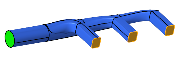
-
Leave the default options in the dialog unchanged then click
on the guide bar to execute the command.
The color of the outlet surfaces change and the list of boundaries on the left are updated. The number of surfaces under each group are shown in the brackets.
Figure 20. 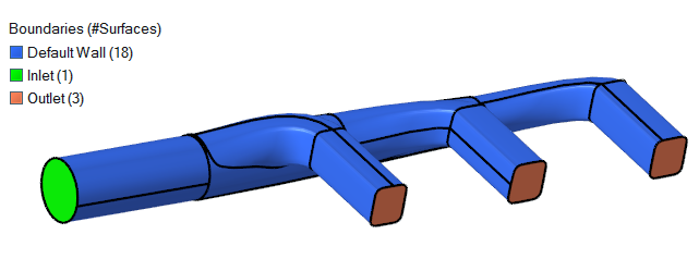
Note:- To update the color of any group, click the colored-square on the left of the group name and select the color of your choice from the palette.
- To update the name of any group, right-click the group name and select Rename from the context menu.
-
On the guide bar, click to exit the
tool.
- Save the model.
Define Mesh Controls
Now that you have assigned the material properties and boundary conditions, you will define the meshing parameters for the model and then generate the mesh.
Define the Surface Mesh Controls
-
From the Mesh ribbon, click the Surface tool.
Figure 21. 
-
Right-click in the modeling window and go to .
Figure 22. 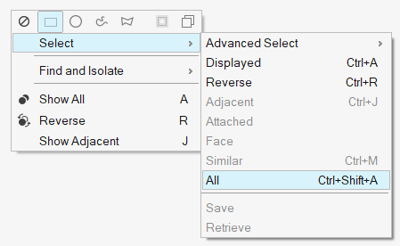
All the surfaces in the model are highlighted and a dialog for surface mesh parameters appears. -
Enter 0.003 m for the Average element size.
Figure 23. 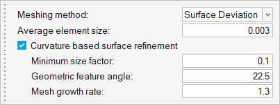
-
Leave the default values for the remaining parameters unchanged then click
on the guide bar to execute
the command.
Define the Boundary Layer Mesh Parameters
-
From the Mesh ribbon, click the Boundary Layer tool.
Figure 24. 
-
Right-click in the modeling window and go to .
Figure 25. 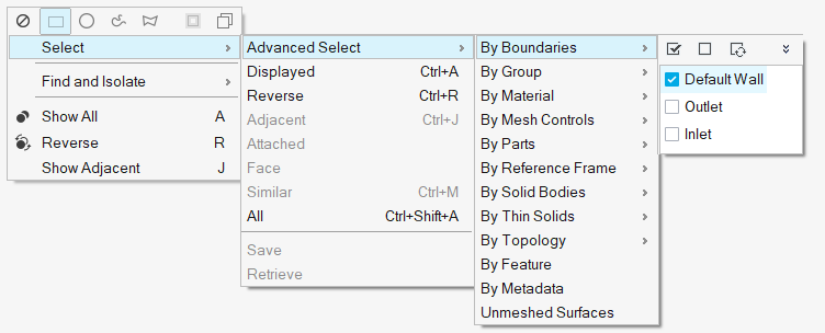
All the wall surfaces are highlighted and a dialog for boundary layer parameters appears. -
Enter the values in the dialog as shown in the figure below.
Figure 26. 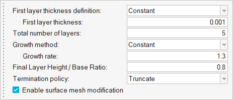
-
On the guide bar, click
to execute the command.
Generate the Mesh
-
From the Mesh ribbon, click the
Volume tool.
Figure 27. 
-
In the Meshing Operations dialog, enter an Average element
size of 0.005 m.
Figure 28. 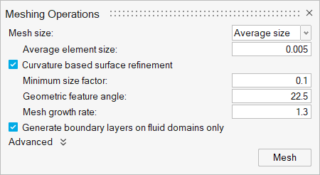
-
Click Mesh.
Once the meshing process has started, the Run Status dialog appears. To view the status of the meshing process, right-click the process row and select View log file.Once the meshing is done, the run status is updated accordingly, and you are automatically moved to the Solution ribbon.
Figure 29. 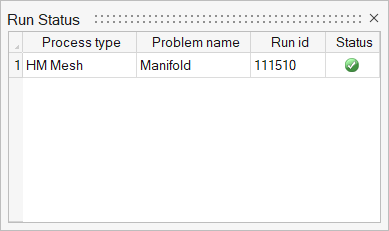
Run AcuSolve
-
From the Solution ribbon, click the Run tool.
Figure 30. 
- In the Launch AcuSolve dialog, verify that the Problem directory and AcuRun path are pointing to the correct location.
- Set the Parallel processing option to Intel MPI.
- Optional: Set the number of processors to 4 or 8 based on availability.
- Deactivate the Automatically define pressure reference option.
- Expand the Default initial conditions menu.
- Deactivate the Pre-compute flow option and enter 2.0 m/s for x-velocity.
- Deactivate the Pre-compute turbulence flow option and enter 1e-5 m2/s for Eddy viscosity.
-
Leave the remaining options as default and click
Run to launch AcuSolve.
Figure 31. 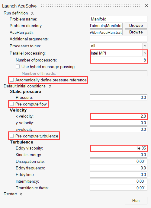
The Run Status dialog opens again and the AcuSolve run appears on the list. -
Right-click on the AcuSolve run and select
View log file.
A summary of the run printed in the dialog indicates that AcuSolve has finished running the simulation. Once the solution is converged, the Status will be updated accordingly.
Figure 32. 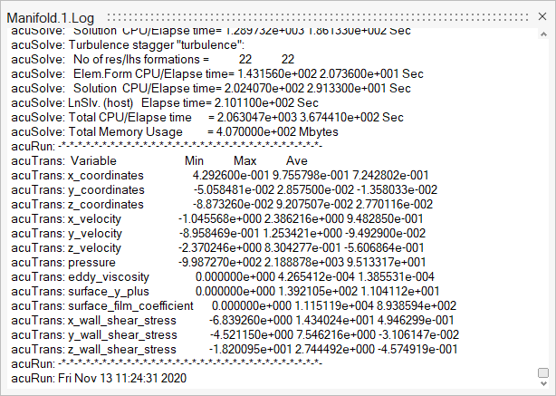
-
In the Run Status dialog, right-click AcuSolve run and select Plot time
history to launch the Plot Manager.
Figure 33. 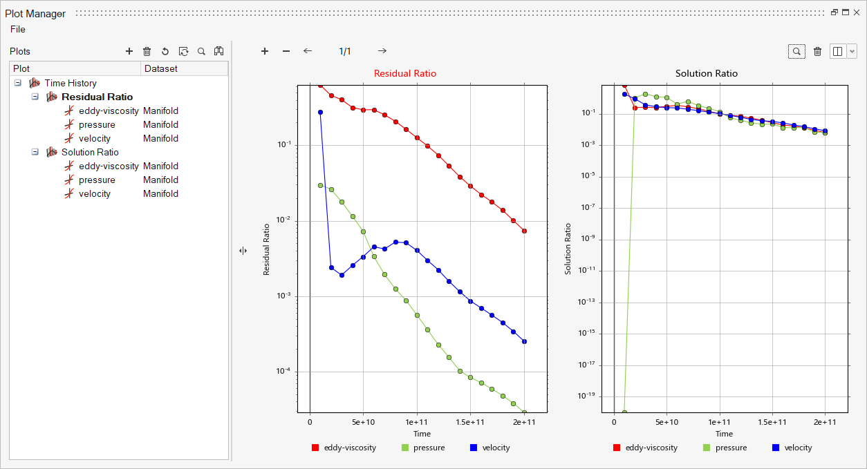
The above plot shows the residual and solution ratios of the equations as the solution progresses through each time step. The convergence check is performed on the residual and solution increment ratios of each equation in the problem. For the residual, the ratio of the residual norm over the norm of the forces of the systems is used. For the solution increment, the ratio of the solution increment norm over the solution norm is used. These ratios are computed separately for each solution field, such as pressure and velocity.
Once the pressure and velocity residual ratios reach a value less than the specified convergence tolerance (0.001), the solution is considered to be converged. By default, the eddy viscosity convergence tolerance is set to a magnitude of one order higher than the specified convergence tolerance (0.01).
Once the pressure and velocity solution ratios reach a value less than the specified convergence tolerance (0.01), the solution is considered to be arrived at steady state. The eddy viscosity solution ratio convergence tolerance is set to a magnitude of one order higher than the specified solution ratio convergence tolerance (0.1).
Post-Process the Results with HyperMesh CFD Post
This part of the tutorial shows you how to work with a steady state solution using HyperMesh CFD Post.
Load the Results
- Once the solution is completed, navigate to the Post ribbon.
- From the menu bar, click .
-
Browse to your working directory. Select the file
Manifold.1.Log and click
Open.
The solid and all the surfaces are loaded in the Post Browser.
Create Pressure Contours on Boundary Surfaces
-
Click the Boundary Groups tool.
Figure 34. 
-
Select all surfaces in the model by holding the left mouse button, dragging,
and drawing a rectangle across the manifold.
Figure 35. 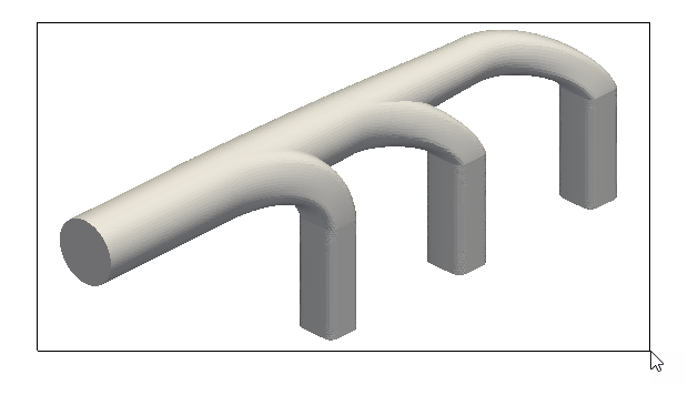
- In the microdialog, set the Display variable to pressure.
-
Activate the Legend toggle and click
 to reset the range.
-
Click
 and set the Colormap Name to Rainbow
Uniform.
and set the Colormap Name to Rainbow
Uniform.
Figure 36. 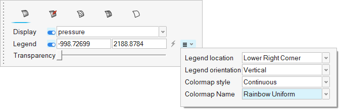
-
Click on the guide bar.
The pressure legend is in Pa.
Figure 37. 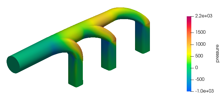
- In the Post Browser, right-click Boundary Group 4 and select Rename. Name it Pressure_plot.
Plot Velocity and Pressure Contours on a Section Cut
-
In the Post Browser, turn off the display of the boundary
surfaces by clicking on the icon next to Flow Boundaries.
Figure 38. 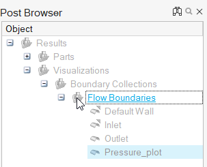
-
Click the Slice Planes tool.
Figure 39. 
-
Select the x-z plane in the modeling window.
Figure 40. 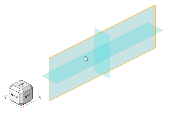
-
In the microdialog, click
 to adjust the plane with the Vector tool.
-
In the Vector tool dialog, click
 to
define the coordinates of the center of plane. Set the value of Y to
-0.015 and press Enter.
to
define the coordinates of the center of plane. Set the value of Y to
-0.015 and press Enter.
Figure 41. 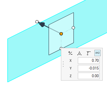
- Press Esc twice.
-
In the slice plane microdialog, click
 to
create the slice plane.
to
create the slice plane.
- In the display properties microdialog, set the Display variable to pressure.
-
Activate the Legend toggle and click to reset the range.
-
Click and set the Colormap Name to Rainbow
Uniform.
Figure 42. 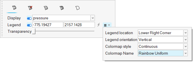
-
Click on the guide bar.
The pressure legend is in Pa.
Figure 43. 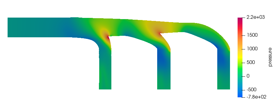
- In the Post Browser, right-click Slice Plane 1 and select Edit.
-
In the microdialog, change the Display variable to
velocity (m/s) then click on the
guide bar.
Figure 44. 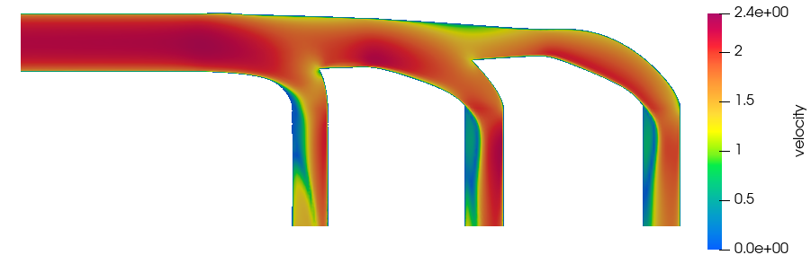
Summary
In this tutorial, you worked through a basic workflow to carry out a CFD simulation and post-process the results using HyperMesh CFD. You started by importing the geometry and meshing the model in HyperMesh CFD. You also set up the model and launched AcuSolve directly from within HyperMesh CFD. Upon completion of the solution by AcuSolve, you post-processed the results in the Post ribbon. You learned how to create contours on the boundary surfaces and section cuts.