
ACU-T: 2100 Turbulent Flow Over an Airfoil Using the SST Turbulence Model
Tutorial Level: Intermediate
Prerequisites
Prior to starting this tutorial, you should have already run through the introductory tutorial, ACU-T: 1000 Basic Flow Set Up. To run this simulation, you will need access to a licensed version of HyperMesh CFD and AcuSolve.
Problem Description

The diameter of the cylindrical bounding volume for the airfoil is set to 500 times the airfoil chord. This large bounding volume is selected to ensure that the farfield boundaries are sufficiently far from the airfoil to prevent any influence of blockage of the domain on the solution.
Since the flowfield near the airfoil is assumed to be turbulent, the SST turbulence model will be used for the simulation. These simulation conditions correspond to a scenario where the boundary layer on the leading edge of the airfoil is tripped with some type of roughness elements to produce a fully turbulent boundary layer over the length of the airfoil.
Start HyperMesh CFD and Create the Simulation Database
- Start HyperMesh CFD from the Windows Start menu by clicking .
-
Click and create a new directory named TubulentAirfoil_SST, or any name of your preference,
and navigate to the directory.
This will be the working directory where all files related to the simulation will be saved.
-
Save the file as Airfoil, or any name of your
preference.
This file will be the database file for this case.
- Click Save to create the database.
Import the Airfoil Geometry
- From the menu bar, click .
- In the Import File dialog, browse to your working directory then select ACU-T2100_NACA0012airfoil.x_b and click Open.
-
In the Geometry Import Options dialog, leave all the
default options unchanged and then click Import.
Figure 2. 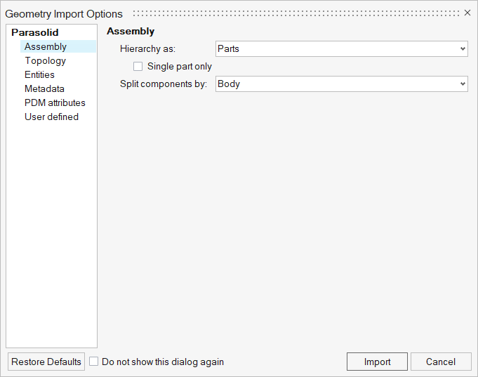
Figure 3. 
Validate the Geometry
-
From the Geometry ribbon, click the Validate tool.
Figure 4. 
The Validate tool scans through the entire model, performs checks on the surfaces and solids, and flags any defects in the geometry, such as free edges, closed shells, intersections, duplicates, and slivers.The current model does not have any of the issues mentioned above. Alternatively, if any issues are found, they are indicated by the number in the brackets adjacent to the tool name.
Observe that a blue check mark appears on the top-left corner of the Validate icon. This indicates that the tool found no issues with the geometry model.Figure 5. 
- Press Esc or right-click in the modeling window and swipe the cursor over the green check mark from right to left.
- Save the database.
Set Up the Problem
Set Up the Simulation Parameters and Solver Settings
-
From the Flow ribbon, click the Physics tool.
Figure 6. 
The Setup dialog opens. -
Under the Physics models setting:
- Verify that the Incompressible option is selected under Single phase flow.
- Set the Time marching to Steady.
- Select SST as the Turbulence model.
Figure 7. 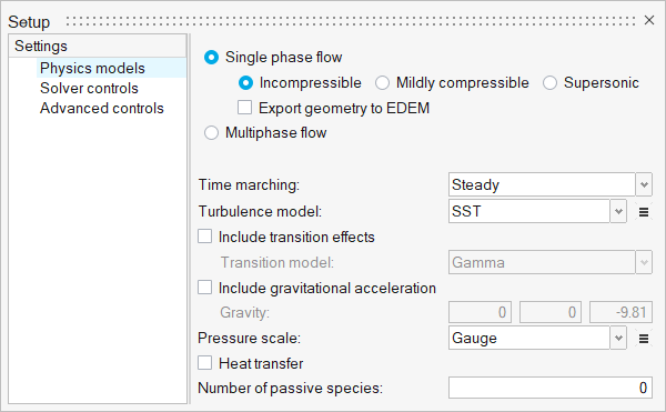
- Click the Solver controls setting.
-
Set the Steady update factor to 0.6, the Steady maximum
steps to 100, and the Convergence tolerance to
0.001.
Figure 8. 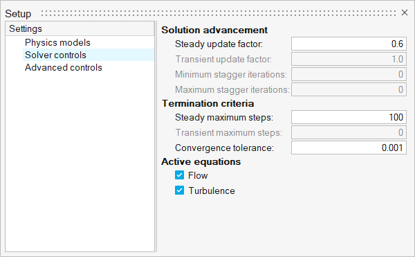
- Close the dialog and save the model.
Verify the Material Selection
-
From the Flow ribbon, click the Material tool.
Figure 9. 
-
Select the model body.
The entire solid is highlighted.
Figure 10. 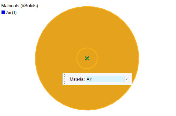
- In the microdialog check that the material Air is assigned by default.
-
Click the Material Library tool to verify the material
properties of air.
Figure 11. 
Air should have the following properties.
- Density: 1.225
- Specific Heat: 1005
- Viscosity: 1.781e-5
- Thermal Conductivity: 0.02521
Figure 12. 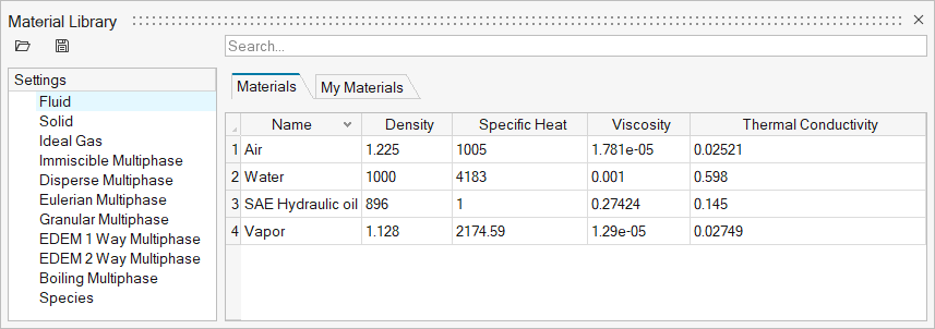
- Close the dialog.
Define Parameters
-
From the Flow ribbon, click the arrow next to the
Setup tool set, then select Parameters.
Figure 13. 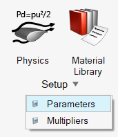
The Parameter Manager opens, which allows you to create variables and expressions which can be used later in the setup. -
Click
 to create a new parameter. Set the Name to xvelocity
and the Expression to 14.48345108.
to create a new parameter. Set the Name to xvelocity
and the Expression to 14.48345108.
-
Create another new parameter: yvelocity =
1.26713777823
Figure 14. 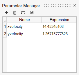
- Close the dialog.
Assign Flow Boundary Conditions
Set a Boundary Condition for the Far Field
-
From the Flow ribbon, click the Far Field tool.
Figure 15. 
-
Rotate the geometry slightly so that the side-surfaces are visible. Click the
two half-side surfaces as shown in the figure below. In the microdialog, type xvelocity and
yvelocity in the respective velocity fields. Accept
all other default parameters.
Figure 16. 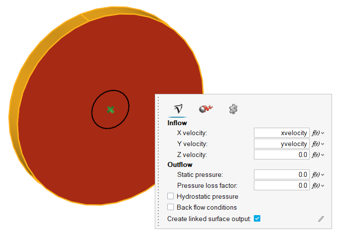
-
Click the Turbulence tab in the microdialog and select External for
the Turbulence flow type. Accept all other default parameters.
Figure 17. 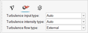
-
Click
 on the guide bar.
The Boundaries legend shows the status of the updated event.
on the guide bar.
The Boundaries legend shows the status of the updated event.Figure 18. 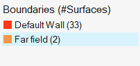
-
On the guide bar, click
 to execute
the command and exit the tool.
to execute
the command and exit the tool.
Set Slip Boundary Conditions
-
Click the Top face of the View Cube to orient the
geometry.
Figure 19. 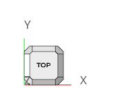
-
Click the Slip tool.
Figure 20. 
-
Select the two surfaces shown in the figure below. Accept all default
parameters in the microdialog.
Figure 21. 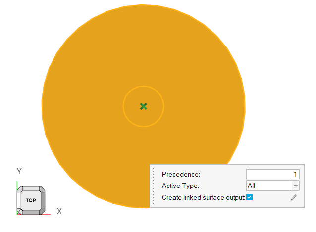
-
Click on the guide bar.
-
Click the Top face of the View Cube once more to orient
the geometry to the bottom view.
Once the view is set, clicking the view again aligns the geometry to the opposite view.
-
Select the surface and accept all default parameters in the microdialog.
Figure 22. 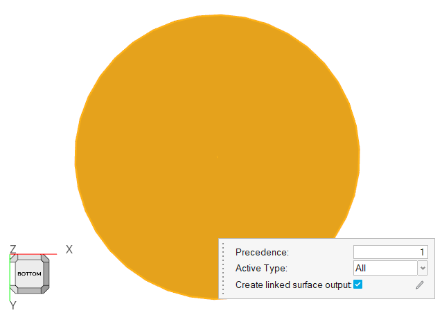
-
Click on the guide bar.
The Boundaries legend should now look like the following:
Figure 23. 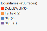
- Click the Bottom face of the View Cube to re-align the geometry with the top view.
- Using the Boundaries legend, rename Slip (2) to +Z slip and Slip (1) to -Z slip.
-
On the guide bar, click
to execute
the command and exit the tool.
Set Wall Boundary Conditions
-
Click the No Slip tool.
Figure 24. 
- Scroll to zoom in so that the airfoil surface is clearly visible.
-
Right-click in the modeling window and choose to select the entire airfoil profile.
Figure 25. 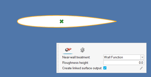
-
Click on the guide bar.
- Using the Boundaries legend, rename Wall (30) to Airfoil.
-
On the guide bar, click
to execute
the command and exit the tool.
- Click the Top face of the View Cube to re-align the model.
Define Mesh Properties
Set Surface Mesh Controls
-
From the Mesh ribbon, click the Surface tool.
Figure 26. 
- Select the outer circular surface shown in the figure below.
-
In the microdialog, set the Average element size to
20 and make sure the Minimum size factor (0.1),
Geometric feature angle (22.5), and Mesh growth rate (1.2) are entered as shown
below.
Figure 27. 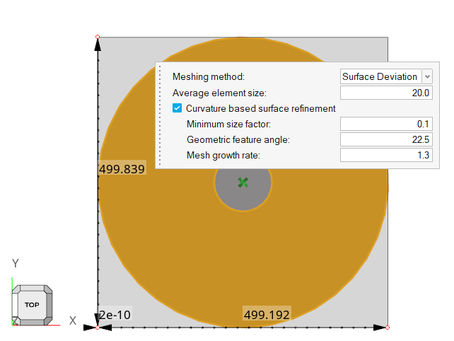
-
Click on the guide bar.
- Select the inner circular surface shown in the figure below.
-
In the microdialog, set the Average element size to
2 and the Minimum size factor to
0.001.
This ensures a smooth transition of mesh size of the airfoil.
Figure 28. 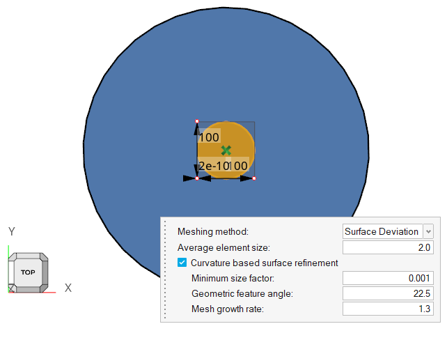
-
Click on the
guide bar.
The Surface Controls legend shows the status of the updated events.
Figure 29. 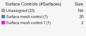
-
On the guide bar, click
to execute
the command and exit the tool.
Set Edge Mesh Controls
-
Click the Edge tool.
Figure 30. 
-
Zoom in on the airfoil.
Figure 31. 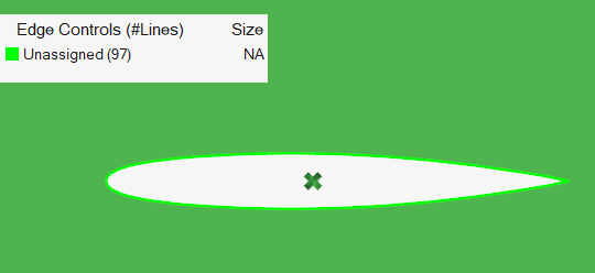
-
Right-click in the modeling window and select .
This also selects the edge of the smaller circle, which will be unselected in the next step. The total number of lines selected is (31).
-
In the microdialog, enter a value of
0.002 for Average element size.
Figure 32. 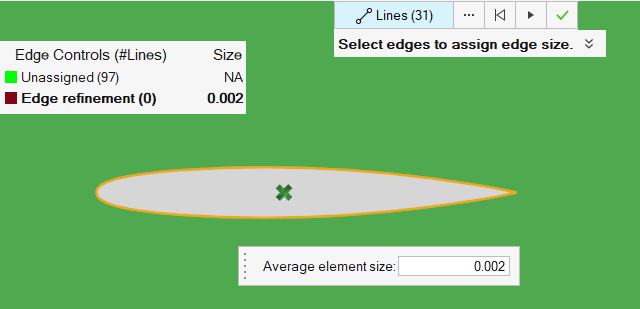
-
Click on the guide bar.
- Zoom out until the edge of the smaller circle appears.
-
Right-click Edge refinement(31) and select
Edit. Keep the cursor on the highlighted edge of the
smaller circular. Press Shift and left click to deselect
the smaller circular edge so that the total lines selected becomes (30).
Figure 33. 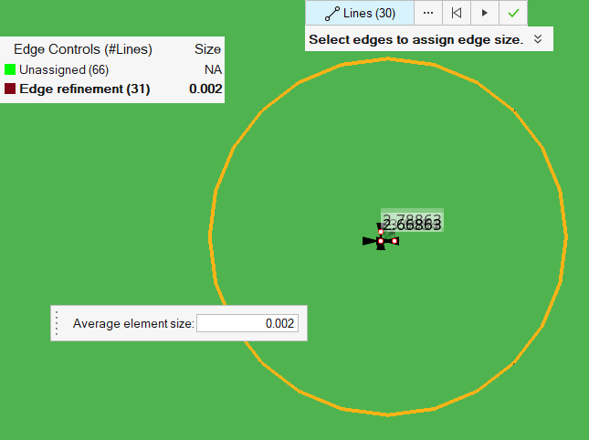
-
Click on the guide bar.
-
Keep the mouse on the smaller circle edge line and click it. Enter the value of
2 for the Average element size.
Figure 34. 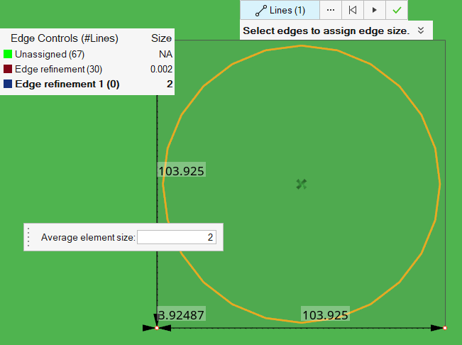
-
Click on the guide bar.
-
Click the Top face of the View Cube.
Figure 35.
-
Select the two outer edges of the outer circle and enter a value of
20 for the Average element size.
Figure 36. 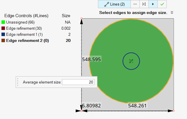
-
Click on the guide bar.
The Edge Controls legend shows the status of the updated events.
Figure 37. 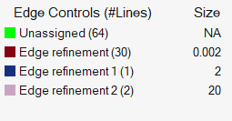
-
On the guide bar, click
to execute
the command and exit the tool.
Set Edge Layer Controls
- Zoom in on the airfoil.
-
Click the Edge Layer tool.
Figure 38. 
-
On the guide bar, click
 besides the Edges selector.
-
In the Advanced Selection dialog, select By
Mesh Controls and enable Edge
refinement.
Figure 39. 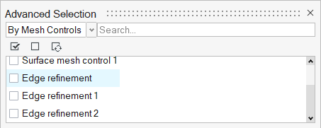
-
In the microdialog, select
Constant for First layer thickness definition. Enter
a value of 0.0001 for First layer thickness and
20 for the Total number of layers for generating mesh
boundary layers. Select Constant for Growth method, enter
a value of 1.2 for Growth rate, and verify a value of
0.8 for Final Layer Height/Base Ratio. Accept all
other default parameters.
Figure 40. 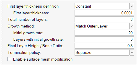
-
Close the Advanced Selection dialog and then click
Parent Surface on the guide bar and select the smaller circular surface (around the airfoil) as shown
below.
Figure 41. 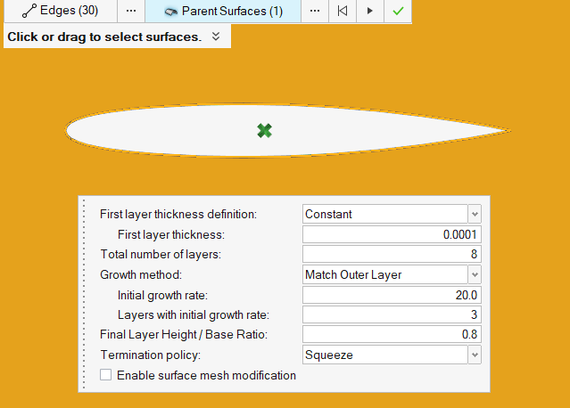
-
Click on the guide bar.
The 2D Boundary Layer Controls legend shows the status of the updated events.
Figure 42. 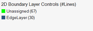
-
On the guide bar, click
to execute
the command and exit the tool.
- Click the Top face of the View Cube.
Set Extrusion Controls
-
Click the Extrusion tool.
Figure 43. 
-
Click Find on the guide bar.
This finds all the solids with mappable surfaces for extrusion.
-
Click Solid (1).
This selects all solids automatically.
- Click Source then select the model surface.
-
In the microdialog, enter a value of
50 for Element Size Along Extrusion and
0.6 for Element size on the surfaces attached to
targets. Accept all other default parameters.
Figure 44. 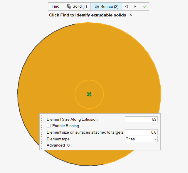
-
Click on the guide bar, observe
the change in the legend, and then click
 .
.
- Save the database.
Generate the Mesh
-
From the Mesh ribbon, click the
Volume tool.
Figure 45. 
The Meshing Operations dialog opens. -
Check that the Average element size is 20. Accept all other default
parameters.
Figure 46. 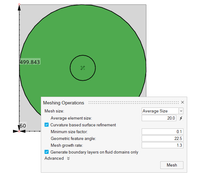
-
Click Mesh.
The Run Status dialog opens. Once the run is complete, the status is updated and you can close the dialog.Tip: Right-click the mesh job and select View log file to view a summary of the meshing process.
-
Click Mesh Only on the View Controls toolbar.
This is used to enable or disable the visualization of mesh.
Figure 47. 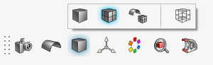
-
Zoom in to check the mesh layers closer to the airfoil surface.
Figure 48. 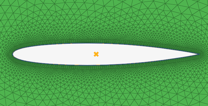
-
Zoom towards the trailing edge of the airfoil to view the mesh.
Figure 49. 
-
From the Home tools, click the Count tool to get the
node and element counts.
Figure 50. 
Figure 51. 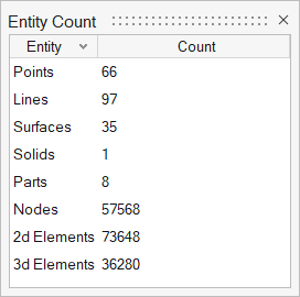
Note: The entity count may differ slightly every time a mesh is generated. - Close the dialog and save the database.
Run AcuSolve
-
From the Solution ribbon, click the Run tool.
Figure 52. 
The Launch AcuSolve dialog opens. - Set the Problem name to NACA0012.
- Set the Parallel processing option to Intel MPI.
- Optional: Set the number of processors to 4 or 8 based on availability.
- Deactivate the Automatically define pressure reference option.
-
Expand Default initial conditions, turn off
Pre-compute flow, and set x-velocity yo
14.48345108 and y-velocity to
1.26713777823. Enable Pre-compute
turbulence.
Figure 53. 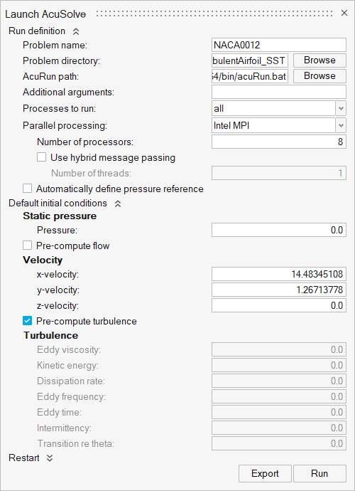
-
Click Run.
Tip: While AcuSolve is running, right-click the AcuSolve job in the Run Status dialog and select View Log File to monitor the solution process.
Post-Process the Results with HM-CFD Post
-
Once the solution is completed, right-click the AcuSolve run in the Run Status
dialog and select Plot time history.
Figure 54. 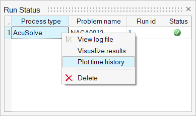
The Plot Manager shows the Residual and Solution Ratios.Figure 55. 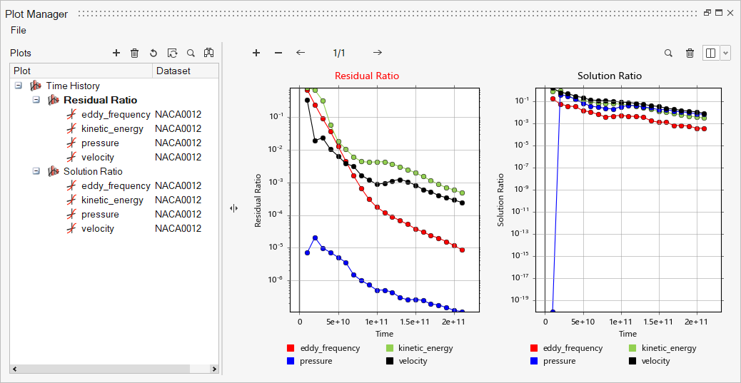
- Close the dialog.
-
Right-click the AcuSolve run again and select
Visualize Results.
You are taken to the Post ribbon.
-
Click the Slice Planes tool.
Figure 56. 
-
Select the x-y plane in the modeling window.
Figure 57. 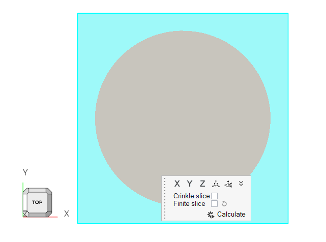
-
Click
 to create the slice plane.
- In the display properties microdialog, set the display to velocity and activate the Legend toggle.
-
Click
 and set the Colormap Name to Rainbow
Uniform.
and set the Colormap Name to Rainbow
Uniform.
Figure 58. 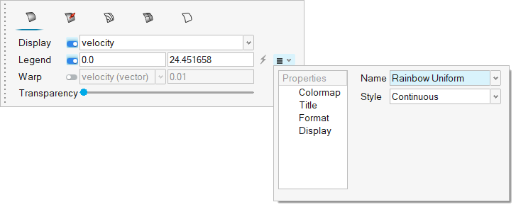
-
Click on the guide bar to
visualize the sqrt eddy period contour.
-
In the Post Browser, click the icon beside Flow
Boundaries to turn off the display for all the flow
boundaries.
Figure 59. 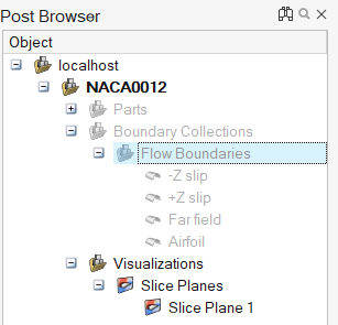
-
On the guide bar, click
to execute
the command and exit the tool.
-
Zoom in on the airfoil to see the contour.
Figure 60. 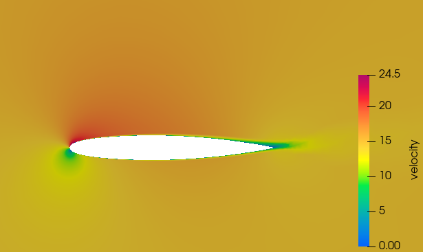
Post-Process to Calculate Flow Coefficients
AcuSolve is shipped with a number of utility scripts to facilitate the pre and post-processing of a problem solved using the solver. You will be introduced to two of these scripts, AcuLiftDrag and AcuGetCpCf in this section, and their usage. These two scripts are focused on aerodynamic simulations as the ones solved in this tutorial.
Run AcuLiftDrag
In the Problem Description section, it was described that the simulation is performed as 2D by including only a single layer of extruded elements in the airfoil span direction. When solving a problem in such a way, the span of the airfoil should be set equal to the thickness of the domain in the extrusion direction. When solving a 3D problem, the actual span of the airfoil should be used.
To execute the AcuLiftDrag script for this position, follow the steps below:- Start AcuSolve Command Prompt from the Start menu by clicking .
- Change the directory to the present problem directory using the cd command.
-
Enter the following command at the prompt:
acuLiftDrag -osis "Airfoil - Output" -aoa 5 -ref_vel 14.54 -chord 1 -ref_rho 1.225 -span 50
The output of the command should look like the image below:Figure 61. 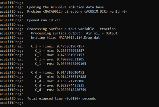
The value C_l corresponds to the lift coefficient, and C_d corresponds to the drag coefficient. The final keyword refers to the respective coefficient values at the last time step of the simulation. The rest of the values provide the basic statistics for these coefficients over all the time steps of the simulation. These statistics are more meaningful if the simulation is transient.
The script also creates the file NACA0012.liftDrag.dat in the problem directory. The file contains the lift and drag data for all the available time steps in a determined tabular arrangement. The first column is the time step, the second column is the lift coefficient, and the third column is the drag coefficient.
AcuGetCpCf
AcuGetCpCf is another utility script used to calculate the coefficient of pressure (Cp) and coefficient of friction (Cf) for the airfoil.
To execute the AcuGetCpCf script for this problem, follow the steps below:
- Start AcuSolve Command Prompt from the Start menu by clicking .
- Change the directory to the present problem directory using the cd command.
-
Enter the following command at the prompt to extract Cp and save it to the file
with the .dat extension.
acuGetCpCf -osis "Airfoil - Output" -type cp -ref_vel 14.54 -ref_rho 1.225 -no_nc -ref_pres 0 –cut_dir z –rad_locs 0.0
The cut_dir option describes the cut plane axis to calculate the Cp and Cf values. rad_locs describes the location of the cut plane on the cut_dir axis. The script prints the minimum and maximum values for the pressure coefficient. It also creates a file, NACA0012.cp.1.dat, in the problem directory. The file contains the pressure coefficient data along the chord of the airfoil. The first column is the x-coordinate along the chord, and the second column is the pressure coefficient.
The output of the command should look like the image below:Figure 62. 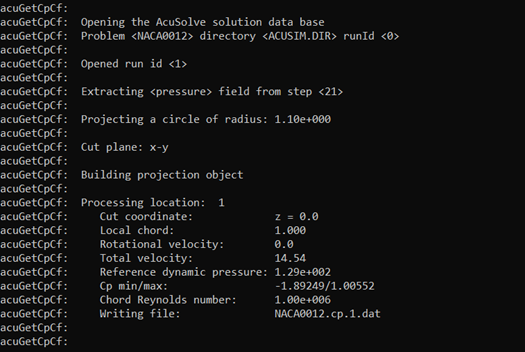
-
Enter the following command at the prompt to plot the variation of Cp along the
airfoil surface, or you can use an external plotting utility to the plot the
data.
acuPlotData -files NACA0012.cp.1.dat -x_col 1 -y_cols 2 -no_pts -ptf -lfmt "-r" -legend AcuSolve -title Cp_variation_along_the_chord -x_label x_along_the_chord -y_label Cp
Figure 63. 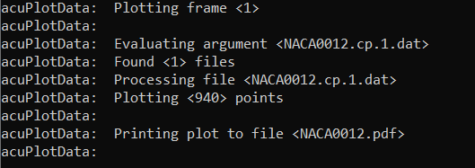
The plotting result is shown below:Figure 64. 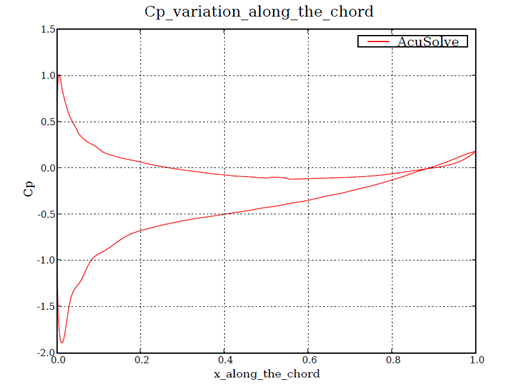
Summary
In this tutorial, you learned how to set up and run a NACA0012 airfoil simulation using HyperMesh CFD and AcuSolve. You started by importing the input CAD file. Next, you assigned the flow boundary conditions and generated the mesh using extrusion. Once the solution was computed, you post-processed the results using HyperMesh CFD Post. Finally, you used a utility script of AcuLiftDrag to calculate the lift and drag coefficients of the airfoil and a utility script of AcuGetCpCfto calculate coefficient of pressure (Cp) and coefficient of friction (Cf). The variation of pressure coefficient along the airfoil surface was plotted using a plotting utility acuPlotData.