
Case Setup
Tutorial Level: Intermediate Use HyperMesh CFD to perform an aerodynamic analysis of a vehicle.
Solution and Environment Selection
Model Transfer to the Case Setup Environment
- Go to and select the HMCFD model Altair_HyperMeshCFD_2025_1_External_Aerodynamics_Case_Setup_Tutorial_Start.hmcfd.
-
Click the Data Transfer Tool. In the guide bar, select
Parts (selected by default). Select all parts in the
model, check the Clear Existing Setup box, and click
Transfer.
Figure 2. 
-
The selected part groups are copied to the Case Setup environment.
Note:
- Alternatively, you may use Part Groups selection. When invoking Part Groups selection, if a part belongs to more than one part group, it will be copied to the Case Setup environment only as part of the first group to which it was assigned. Only actual part groups are transferred. Parts which are not assigned to a part group will be ignored on transfer.
- When invoking Part selection, all selected parts are
transferred.Tip: You may also import mesh and CAD files directly from the HMCFD Case Setup environment through . You may manually switch to the Case Setup environment, by selecting Case Setup from the drop-down to the right of View.
Case Environment Setup
-
Invoke the Model Browser and Property
Editor from the View menu.
Both open on the left side of the modeling window.
-
Change the model projection to Orthographic.
Figure 3. 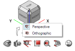
Baffles
Parts represented by surfaces with no thickness where both parts of the surface are exposed to the flow must be identified as baffles. Alternatively, they may be thickened in the Geometry Repair environment. The Geometry Repair environment offers multiple tools to find baffle parts/surfaces/elements in a model.
- In the Model Browser, click on the magnifying glass to open the search bar.
- Type “Baffle”.
- Click on the Underbody_Shield_Rear_Baffle part.
- In the Property Editor, check the box under .
- Clear the search bar in the Model Browser to show all parts.
Model Organization
- From the Model Browser, type Porous_Media in the search bar.
- Highlight all shown parts, then right-click and select New Assembly.
- Rename the newly created assembly as Porous_Media.
- Clear the search bar in the Model Browser.
- Repeat steps 1 to 4 for Body_Exterior, Chassis, Cooling_Module, Electronics_Module, Patch (rename as Patches), Steering (rename as Steering Module), Suspension (rename as Suspension_Module), Underbody, VREV (rename as VREVs), Monitor_Surface (rename as Monitor_Surfaces), Wheel (rename as Wheels), HVAC (rename as HVAC_Module), Fan (rename as Fan_Assembly). Only select those parts which are not inside another assembly.
- In the Model Browser, right-click on the Model assembly and select New Assembly.
- Rename the newly created assembly as Main.
-
Collapse all other assemblies, then select, drag, and drop them into the
Main assembly.
Note: When dealing with many parts, this process may be slow. In that case, try dragging the assemblies one at a time into the Main assembly.
- From the Model Browser, type RL7 in the search bar.
-
Highlight all shown parts, then right-click and select New
Assembly.
An assembly is created within the Underbody assembly.
- Rename the newly created assembly as RL07.
- Right-click on the Main assembly and click Isolate to isolate the parts contained within the Main assembly.
Model Dimensions
The ultraFluidX 2023.0 Setup guidelines for vehicle aerodynamics, provides various setup recommendations which rely on the model dimensions and position. HMCFD’s Case Setup environment allows you to gather this information through the GUI and the Python Window.
Python Window
- Open the Python Window by going to or pressing F4 on your keyboard.
-
Execute the following:
- from hwx import inspire
- model = inspire.getActiveModel()
-
model.axisAlignedBoundingBox
Output: Box(x=4.96514, y=2.1354, z=1.42625)
-
model.axisAlignedBoundingBox.minMax
Output: (Point (-0.9074339866638184, -1.0676989555358887, -0.010730000212788582),
Point (4.057706832885742, 1.0676989555358887, 1.415518045425415))
GUI
- Select all parts in the viewer.
-
Click on the Measure tool.
Figure 4. 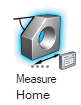 A bounding box fitted to the selected parts will show along with its X, Y, Z dimensions.
 - Given that z-min is zero, the vehicle’s centerline is at y = 0, and the vehicle can be assumed to be symmetric about the Y plane, we can derive the Y and Z mins and maxes from this data. One way to find x-min is to use the RL Box creation tool.
- Click on the .
- Click on any surface of the body.
- From the , set the Length to 4.965 (shown by the Measure tool).
- Orient your model to the Right view.
- Drag the box along X until the front and rear of the box appear to be just touching the front and rear surfaces of the model respectively.
- Note the x-min and x-max values in the .
- Delete the box by right-clicking on the part in the .
Define Wind Tunnel
-
From the Setup ribbon, click the Edit Tunnel tool.
Figure 5. 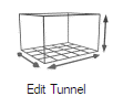 A tunnel is generated around the model. The tunnel size is automatically set based on the best practices for vehicle simulations.
 -
In the Property Editor, go to and set the inflow speed to 38.889
m/s.
Tip: Tip You can also double-click on the large arrow at the bottom of the wind tunnel to set the wind speed.
-
From either Tunnel Properties in the Property
Editor or the micro-dialogs in the modeling window, modify the
dimensions of the wind tunnel.
- Enter a value of 79.44 m for the Length.
- Enter a value of 53.375 m for the Width.
- Enter a value of 29.945 m for the Height.
-
From Tunnel Extents in the Property
Editor.
- Enter a value of -24.826 m for the X Min.
Advanced Tunnel Setup (Belts & Patch)
The “standard” external aerodynamics wind tunnel setup calls for a full moving ground configuration. Modelling setups which emulate those in wind tunnels are possible using the Belts Tool together with the Ground Patch as described below.
-
From the Property Editor, enable the checkbox under .
Note: Enabling Boundary Layer Suction sets the boundary condition of the ground upstream of the boundary layer suction line (blue dotted line) to a slip wall boundary condition. Enabling boundary layer suction is recommended whenever static ground conditions apply to the simulation. This includes moving belts surrounded by a static ground region.
-
From the Property Editor, enable the checkbox under .
Note: Enabling Ground Patch sets the boundary condition of a region of the ground – which extends from the center of the vehicle to upstream, downstream, and to each side a pre-set distance away from the vehicle based on the vehicle’s dimensions and belt dimensions in whenever applicable – to a zero-velocity non-slip wall boundary. Enabling the ground patch is recommended whenever static ground conditions apply to the simulation. This includes moving belts surrounded by a static ground region.
Figure 6. 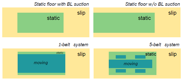
- Press Esc or right-click in empty space to exit the tool.
- Select the Wind Tunnel and hide it with the H shortcut key.
Identify Parts
Use the Identify Parts tool to define types of parts like wheels, heat exchangers or body panels, which require specific modeling techniques for the CFD run. During import, all parts are identified as body by default. This applies a zero-velocity wall boundary condition for the CFD analysis. Besides the default Body identification, the Identify Parts tool allows you to identify parts as a Heat Exchanger, Wheel or Fan.
Wheels
When modeling a wheel, a wall boundary condition is prescribed, and – when the Rotating wheels option is enabled () – a rotational velocity – based on the distance from the axis of rotation to the ground – is applied. Once you select the parts forming the wheel assembly, parameters like the center of rotation, axis of rotation, and angular velocity (in RPM) are computed automatically (these may be overwritten by the user by disabling “Auto Calculate” – see Step 6). If multiple parts are selected, the parts will be grouped into one or more wheels. For example, if you select the brake disc, the rim and the tire of the left front wheel, all three parts will be identified as wheel_1. If you also select the rim and the tire of the left rear wheel, those parts will be grouped into wheel_2.
Identification
-
To view only the parts that make up the wheels, you will need to hide the rest
of the parts.
- In the , select the Wheels assembly.
- Right-click and select Isolate from the context menu or press I to isolate the wheel geometry.
-
From the Setup ribbon, click the Identify
Parts tool.
Figure 7. 
-
From the secondary tool set, click the Create Wheel
tool.
Figure 8. 
-
Select all Wheels parts.
Figure 9. 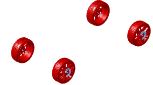
- Click on the parts now identified as wheels in the Model Browser.
- In , ensure that Auto Calculate is enabled.
- Press Esc or right-click in empty space to exit the tool once all the wheels have been identified.
Rotating Wheels
-
From the Setup banner click on the Run tool.
Figure 10. 
-
From the setup micro-dialog, under Analysis setup,
enable Rotating wheels (it is enabled by default). If
left unchecked, the wheels will be identified as such, but a zero velocity
non-slip boundary condition will apply.
Note: For the Wheel Setup, either MRF or OSM option, VREVs surface normals must be pointing outwards. Isolate the VREVs assembly, click on the Normals tool and make sure all the surface normals have the correct orientation. If needed, click on the surfaces that with the wrong surface normals orientation to fix them. Exit the tool and from the Model Viewer, isolate the Main assembly to show the full vehicle model.
Moving Reference Frame (MRF) Wheel Setup
Moving Reference Frame (MRF) regions define a volume in which the governing equations are solved in a rotating reference frame. This transformation of the equations can lead to higher accuracy for rotating bodies due to the addition of centrifugal and Coriolis forces. A closed volume of revolution (VREV) is generated in HMCFD for each MRF region.
- If parts other than the wheels are currently displayed, isolate the wheels by repeating Step 1.
- From the Setup ribbon, click the Identify Parts tool.
-
From the secondary tool set, click MRF tool. A guide bar appears below the
tool.
Figure 11. 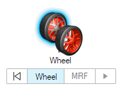
-
Click on any part of the front-left wheel which was identified as
Wheel in steps Step 1-5.
The entire wheel group is selected.
- From the Model Browser, select and Show the part named VREV_Wheel_Spokes_Front_Left.
- On the guide bar, click MRF.
-
From the display window, click on
VREV_Wheel_Spokes_Front_Left (the disk on the
front-left wheel) to identify it as the MRF region.
Figure 12. 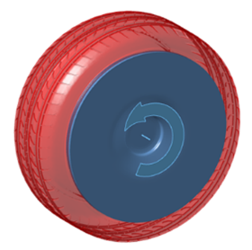 The region is highlighted blue.
 - Click Play on the guide bar to confirm your selection.
- Repeat the above process for the other wheels, using their respective VREV parts.
-
From the Model Viewer, isolate the
Main assembly to show the full vehicle model.
Tip: Use the Tab key to cycle between Wheel and MRF selections. Click Back on the guide bar to clear a selection.
- The angular velocity and center of rotation of the rotating frames are extracted from the wheel definitions. Tip:
Overset Mesh (OSM) Region Wheel Setup
Overset Mesh (OSM) Regions define a volume in which all voxels and surface elements contained within are rotated about its axis. This transformation of the geometry can lead to higher accuracy for rotating bodies as it more closely approaches the intended state as compared to wall velocity BC and MRF methods. A closed volume of revolution (VREV) is generated in HMCFD for each OSM region.
Due to reasons related to legacy, the OSM workflow utilizes the Fan identification tool.
- If parts other than the wheels are currently displayed, isolate the wheels by repeating Step 1.
- From the Setup ribbon, click the Identify Parts tool.
-
From the secondary tool set, click Fan tool. A guide panel appears, and a
selector tool is activated.
Figure 13. 
- Click on the Wheel_Spokes_Front_Left part.
- From the select Overset.
- From the Model Browser, select and Show the part named VREV_Wheel_Spokes_Front_Left.
- From the Fan Guide panel, press the Select button.
- From the display window, click on VREV_Wheel_Spokes_Front_Left (the disk on the front-left wheel) to identify it as the OSM region. The region becomes transparent.
- Flip the rotation of the OSM region to match that of the wheels by pressing the +/- button in the Axis micro-dialog.
- From the Axis micro-dialog, set the RPM to 1031.569 to match the auto-calculated RPM of the wheels. Alternatively, you may edit the RPM value from the Property Editor.
-
From the Fan Guide panel, enable Mesh
Controls and set the Refinement Level
value to 6.
This will ensure that voxels within the OSM Region are at most the size of Resolution Level 6 (RL06) voxels.
-
From the Fan Guide panel, enable Interface
Refinement and set the Refinement Level
value to 7. This will ensure that voxels along the
interface (as represented by the elements of the VREV part) of the OSM Region
are at most the size of Resolution Level 7 (RL07) voxels.
Note: In certain cases – most commonly when dealing with high performance vehicle – the gap between the wheel spokes and the brake caliper may be small enough to require higher resolution at the interface. As a rule of thumb, you should aim to fit a minimum of 9 voxels in this gap: 6 from the surface of the spokes (the rotating geometry), and 3 from the surface of the caliper (the stationary geometry). You should never fit less than 4.5 voxels from the rotating geometry and/or 1.5 voxels from the static geometry.
- Click Play on the Fan Guide panel to confirm your selection.
- Repeat the above process for the other wheels, using their respective VREV parts.
-
From the Model Viewer, isolate the
Main assembly to show the full vehicle model.
Note: The split intersecting part option included in the Fan Guide panel was not used here because the parts used in this example were already split in the Geometry Repair environment of HMCFD prior to transferring the model to the Case Setup environment. This is the recommended process. Please refer to the Geometry Report portion of the External Aerodynamics Tutorial for details on how to perform these operations.
Heat Exchangers
-
To view only the parts that make up the heat exchangers, you will need to hide
the rest of the parts.
- In the , select the Porous_Media assembly.
- Right-click and select Isolate from the context menu or press I to isolate the wheel geometry.
- From the Setup ribbon, click the Identify Parts tool.
-
From the secondary tool set, click the Heat Exchanger
tool.
Figure 14. 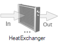
-
The Heat Exchanger Inlet Selection Tool should be
automatically selected. If it is not, click on the In
arrow of the Heat Exchanger Tool.
Figure 15. 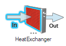
- From the graphics area, click on the part named Porous_Media_Transmission_Oil_Cooler_Inlet to identify it as the inlet of that heat exchanger.
-
Click on the Heat Exchanger Wall Selection Tool.
Figure 16. 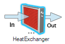
- Click on the part named Porous_Media_Transmission_Oil_Cooler_Walls to identify it as the wall of that heat exchanger.
-
Click on the Heat Exchanger Outlet Selection Tool.
Figure 17. 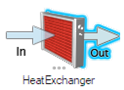
- Click on the part named Porous_Media_Transmission_Oil_Cooler_Outlet to identify it as the outlet of that heat exchanger.
-
Create a second heat exchanger by clicking the plus button in the Heat
Exchanger Dialog.
Figure 18. 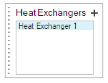
- Repeat Steps 4-10 to setup the other two heat exchangers.
- Press Esc or right-click in empty space to exit the tool.
- From the Model Browser, select each part identified as heat exchanger. From the Property Editor, enter 100 in and 300 in . Repeat this step for the other two heat exchangers.
-
From the Model Viewer, isolate the Main assembly to show
the full vehicle model.
Note: If a heat exchanger is not split into separate Inlet, Outlet, Wall parts, you may identify all its parts as Inlet. However, since the direction won’t be auto-calculated, you will have to enter the flow direction vector in the Property Editor under Permeability Direction.
Adjust Heave
-
From the Setup ribbon, click the Adjust Heave
Tool. The Adjust Heave micro-dialog opens
and the z-distance of each axle axis to z = 0 is displayed in the viewer.
Figure 19. 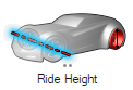
- Click on the distance value for the front axle. The Height input micro-dialog appears. Set the Height value to 0.35 m.
- Click on the distance value for the rear axle. The Height input micro-dialog appears. Set the Height value to 0.35 m.
- Exit the Adjust Heave Tool by clicking on the green checkmark on the Adjust Heave micro-dialog.
Define the Belt System (Advanced)
Once the wheels are defined, the belt tool will automatically create belt patches to fit the body and wheels of the vehicle.
-
From the Setup ribbon, click the Belt
System tool. By default, five patches are created on the wind
tunnel floor to model the belt system.
Figure 20. 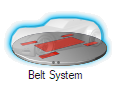
- From , rename the belts as Belt_Front_Left, Belt_Rear_Left, Belt_Front_Right, Belt_Rear_Right, and Belt_Center accordingly.
- You may edit the size and parameters for the belts from the Property Editor.
- From , select Belt_Center.
- From the Property Editor, uncheck the box for .
- Copy the value in .
- From the Model Browser, click on the Wind Tunnel.
- From the Property Editor, activate , change the reference to Origin, and paste the copied value into . This will set the Wall Boundary Condition of the ground upstream of that location to Slip Wall.
- Make sure is also enabled and its length has been adjusted accordingly with the new BL Suction location.
- Click on the icon to hide the belts.
Define Mesh Controls
Use the Mesh Controls tool to define regions with a user-defined volume element size.
All other mesh controls in the model are defined relative to the far field size and must be a power of 2 of the far field size. For example, if you define a far field mesh size of 1 m, the available refinement sizes will be 0.5 m, 0.25 m, 0.125 m, etc.
Far Field Element Size
-
From the Setup ribbon, click the Mesh Controls
tool.
Figure 21. 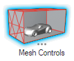
-
From the secondary tool set, click the Far Field tool.
Figure 22. 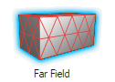
- Verify the element size is set to 0.192 m.
Transition Layers
-
From the Setup ribbon, click the Advanced Meshing
Parameters tool.
Figure 23. 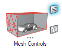 The ultraFluidX Mesh Controls Dialog opens.
 -
Set the value of to 8.
This instructs the solver to ensure that each resolution layer is at least eight levels thick.
- Close the ultraFluidX Mesh Controls dialog.
Box Refinement Zones
- From the Setup ribbon, click the Mesh Controls tool.
-
From the secondary tool set, click the Body Box Zone
tool.
Figure 24. 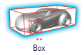
-
Select any location on the model body.
A new refinement zone is generated around the body and the Box Zone micro-dialog appears.
- From the Box Zone micro-dialog, enter a value of 5 for Level, 6.951 m for Length, 2.776 m for Width, 1.783 m for Height, and press Enter.
- In the Property Editor, set to -1.407 m and rename your box by setting to RL05_Box.
-
From the Box Zone micro-dialog, click
Plus.
A second box refinement zone, one level coarser is generated.
-
Repeat Steps 4-6 for zones 4, 3, 2, and 1 using the values provided in the
table below.
Table 1. Level Name Length Width Height X Min 4 RL04_Box 8.937 m 3.416 m 2.139 m -1.904 m 3 RL03_Box 11.420 m 4.270 m 2.496 m -2.400 m 2 RL02_Box 14.895 m 5.338 m 2.852 m -3.390 m 1 RL01_Box 24.825 m 6.405 m 3.565 m -5.880 m Note: The Length, Width, Height, and X Min values the table above are calculated from equations provided in the ultraFluidX 2023.0 Setup guidelines for vehicle aerodynamics.Note: Alternatively, you may use the Part Box Zone tool to prescribe a refinement zone around a single part.Figure 25. 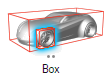
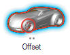
Offset Refinement Zones
As opposed to the Box tool, which creates a box-shaped refinement zone, the mesh refinement patterns of the Offset tool follow the contour of the body itself. This creates refinement around the body where it is needed most, eliminating unnecessary refinement that may result from a box-shaped zone.
Body
- From the Setup ribbon, click the Mesh Controls tool.
-
From the secondary tool set, click the Body Offset tool
to create an offset zone around all parts identified as Body, Wheel, Fan, and
Heat Exchanger.
-
Select a point on the model body.
The Offset Tool micro-dialog opens.
- From the Offset Tool micro-dialog, use the drop-down menu to change the method from Distance to Layers.
-
Set Layers to 12 and
Level to 6.
Tip: You can also change the distance or number of layers by interactively dragging the slider in the modeling window.
- From the Property Editor, rename the offset by setting the value of to RL06_Offset.
Parts
- From the Model Browser, multi-select all parts within the and assemblies. Press I on your keyboard to isolate the selected parts.
- From the Setup ribbon, click the Mesh Controls tool.
-
From the secondary tool set, click the Part Offset tool
to create an offset zone around selected parts.
Figure 26. 
-
From the Display Window, rubber-band select all displayed
parts.
The Offset Tool micro-dialog opens.
- From the Offset Tool micro-dialog, use the drop-down menu to change the method from Distance to Layers.
- Set Layers to 8 and Level to 7.
- From the Property Editor, rename the offset by setting the value of to RL07_Offset.
- From the Model Viewer, isolate the Main assembly to show the full vehicle model.
Define the Outputs
-
From the Setup ribbon, Run group,
click the Run tool.
Figure 27.
The Run dialog opens. - From the Run dialog, verify the value is set to 38.889 m/s as per Step 2.
-
Click on the lightning bolt button for .
Note: The value of is linked to the value of as they represent the same value in two different units: timesteps and seconds, respectively.This automatically sets the value to the time it would take for flow traveling at the inflow speed to traverse the length of the vehicle 30 times as per the ultraFluidX 2023.0 Setup guidelines for vehicle aerodynamics
- Note the value of for future use.
- Close the Run dialog.
-
From the Setup ribbon, Output group,
click the General Output Tool.
Figure 28. 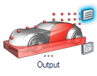 The ultraFluidX Output Controls dialog opens.
 -
From the ultraFluidX Output Controls dialog, click on the
lightning bolt button for .
This automatically sets the value to the time it would take for flow traveling at the inflow speed to traverse the length of the vehicle 15 times as per the ultraFluidX 2023.0 Setup guidelines for vehicle aerodynamics.
-
Set the value for to 0.174091 s and that of to 229.
Note: Ideally, we want to synchronize the output frequency with the averaging window size and averaging start time. In this case, a total runtime of 5,038 timesteps (3.83 s) can be factored into 22 * 229, leaving 2,519 timesteps (1.915 s) for the first 15 flow-passes and 2,519 timesteps for averaging. The final 15 flow-passes may be further divided into 11 windows of 229 timesteps (0.174091 s).
-
Click on the hamburger menu of .
The General Output Field Variables dialog opens.
- From the General Output Field Variables dialog, set the value of Start iteration to 2519.
- If the OSM approach for the wheels from Wheels is being used and the filetype for the results is Ensight, enable the displacement and field variables.
- Close the General Output Field Variables dialog.
-
From the ultraFluidX Output Controls dialog, set the value
of to 2.
Note: This will limit the number of saved frames for the Full and Surface datasets to 2 by overwriting the earliest written frame as a new one is output as per the output frequency starting at the start iteration.
- Enable (and Y and Z) and set the value of each to 100.
- From the ultraFluidX Output Controls dialog enable the Coarsen option.
- Set the Refinement level to 5 and Target refinement level to 2.
- Close the ultraFluidX Output Controls dialog.
Section Cuts
-
From the Setup ribbon, click the
Output tool.
Figure 29. 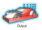
-
From the secondary tool set, click the Section Cut
tool.
Figure 30. 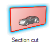 The Section tool micro-dialog opens and the X, Y, and Z planes are highlighted in the viewer.
 -
Click on the Y-Plane.
The Plane Dialog opens.
- From the Plane dialog, use the pulldown menu to change the start method from Start Iteration to Start Time, and set the start time value to 3.73 s to capture the last 0.1 s of the simulation.
- From the Plane dialog, use the pulldown menu to change the output method from Output frequency to Hz, and set the Target frequency value to 1000 Hz.
- Click on the hamburger menu on the upper right corner of the Plane dialog to open the list of output variables and uncheck all time-averaged variables.
- Click on the expand icon on the upper right corner of the Plane dialog to show the Length and Width fields. Set the Length value to 8 m.
- Click on the move tool icon on the upper right corner of the Plane dialog to open the move tool. Drag the plane along the X-Axis by 1.043 m and along the Z-Axis by 0.188 m.
- Close the Section Cut tool by pressing on the green checkmark button on the Section Cut micro-dialog.
-
From the , rename the newly created Section Cut to
Section_Cut_Y_Center and hide it.
Tip: Double click the edges of the section cut in the modeling window to resize the plane.
Probes
Surface Probes
- From the Model Browser, multi-select all parts within the assembly. Press I on your keyboard to isolate the selected parts.
- From the Setup ribbon, click the Output Tool.
-
From the secondary tool set, click the Surface Probes
Tool.
Figure 31. 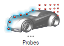 The Surface Probes micro-dialog opens.
 -
From the viewer window, rubber-band select all the
displayed parts.
The Probes dialog opens.
- From the Probes dialog, set the Start iteration value to 2519.
-
On the upper left corner of the viewer window, a list of surface probes sets
will show. Right-click on the set that was just created
(there should only be one) and click on Probes table.
The Probes Table opens.
-
Press the open icon on the Probes Table, navigate to the
Surface_Probes.csv file provided, and click Open.
The probes are imported to the selected set.
- Close the Probes Table.
- Close the Surface Probes Tool by pressing on the green checkmark button on the Surface Probes micro-dialog.
- From the , rename the newly created Surface Probe set to Surface_Probes and hide it.
- From the Model Viewer, isolate the Main assembly to show the full vehicle model.
Volume Probes
- From the Setup ribbon, click the Output Tool.
-
From the secondary tool set, click the Volume Probes
Tool.
Figure 32. 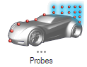 The Volume Probes micro-dialog opens.
 -
From the viewer window, click on any point in space.
A volume probe is created and the Probes Dialog opens.
- From the Probes dialog, set the Start iteration value to 2519.
-
On the upper left corner of the viewer window a list of volume probes sets will
show. Right-click on the set that was just created (there should only be one)
and click on Probes table.
The Probes Table opens.
-
Press the open icon on the Probes
Table, navigate to the Volume_Probes.csv
file provided, and click Open.
The probes are imported to the selected set.
- Delete the first row in the Probes Table as this was the one created by randomly clicking in space.
- Close the Probes Table.
- Close the Volume Probes Tool by pressing on the green checkmark button on the Volume Probes micro-dialog.
- From the , rename the newly created Volume Probe to Volume_Probes and hide it.
Monitor Surfaces
- From the Setup ribbon, click the Output Tool.
-
From the secondary tool set, click the Monitor Surface
Tool.
Figure 33. 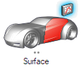 The Monitor Surface micro-dialog opens.
 -
From the viewer window, click on the
Monitor_Surface_Grille part. Tip:
Tip: Isolate the part before selecting for easier access.The part is assigned as Monitor Surface and Monitor Surface dialog opens.
- From the Monitor Surface dialog, for the Visual settings, set the Start iteration value to 2519 and the Output frequency to 229.
- Close the Monitor Surface Tool by pressing on the green checkmark button on the Monitor Surface micro-dialog.
- From the , rename the newly created Monitor Surface to Monitor_Surface_Grille and hide it.
Turbulent Sources
Turbulence generators (TGs) are used to force laminar to turbulent behavior of the boundary layer. They may be used to calibrate the turbulent boundary layer thickness in the wind-tunnel and force laminar-turbulent transition on flat surfaces.
Ground (Advanced)
When not using the “Standard” ground setup of full moving ground, the use of turbulence generators near the boundary layer suction region is recommended.
-
From the Setup ribbon, click the Turbulence
Source Tool.The
Turbulence Source micro-dialog opens.
-
From the viewer window, click on any part.
A turbulence source is created and the Turbulence Source dialog opens.
- From , click on the newly created Turbulence Source.
- From the Property Editor, set the value to Turbulence_Source_Ground to rename the newly created Turbulence Source.
- Set the values to 7.477 m, 3.2 m, and 0.024 m respectively.
- Set the values to -2.159 m, -1.608 m, and 0 m respectively.
- Deactivate Auto Calculate for and .
- Set to 0.01, 0.012 m and 800 respectively.
- Close the Turbulence Source Tool by pressing on the green checkmark button on the Turbulence Source micro-dialog.
-
Hide the Turbulence_Source_Ground part.
Note: Parameter values specified for the ground turbulence source were calculated as per the ultraFluidX 2023.0 Setup guidelines for vehicle aerodynamics. This region is intended to accurately develop the boundary layer in the areas of the static ground near the vehicle downstream of the boundary layer suction.
Bulk (Optional)
For flat surfaces and certain smooth designs, the boundary layer might remain artificially pseudo-laminar. In such case, TGs may be added in the bulk and in front of the flat surface to force the laminar-turbulent transition and obtain a more realistic boundary layer development.
-
From the Setup ribbon, click the Turbulence
Source Tool.
The Turbulence Source micro-dialog opens.
-
From the viewer window, click on the hood of the
vehicle.
A turbulence source is created, and the Turbulence Source dialog opens.
-
Click on the expand icon on the upper right corner of
the Turbulence Source dialog to show the Length, Width, and
Height fields.
- Set the Length, Width, and Height values to 1 m, 1.906 m, and 1 m respectively.
- Click on the hamburger menu on the upper right corner of the Turbulence Source dialog to expose additional parameters and set the value of Number of Eddies to 800.
- From , click on the newly created Turbulence Source.
- From the Property Editor, set the value to Turbulence_Source_Front to rename the newly created Turbulence Source.
- Set the values to -1.1 m and 0 m respectively.
- Close the Turbulence Source Tool by pressing on the green checkmark button on the Turbulence Source micro-dialog.
- Hide the Turbulence_Source_Front part.
Export Solver Deck
-
From the Setup ribbon, Run group,
click the Run tool.
The Run Dialog opens.
- From the Run dialog, set the value of Name of run to Aurora.
- Set the Run path to a path of your choosing.
-
Click on the Export button.
One XML, one STL, one ZIP, one INFO, and two CSV files are created. The ZIP file is a compressed version of the STL file. All but the INFO and STL files are required as solver input.
Submit Job
- Follow Steps 1-3.
-
Click Run.
Note: If you are running HyperMesh CFD on a Linux system with a supported GPU, a solver run is started. If you are running HyperMesh CFD on a Windows system, you'll need a Linux installation of ultraFluidX available for running the solver.Note: To run the solver from Windows:
- Click Export. This generates an stl and xml file in the run directory.
- Copy the stl and xml files to the Linux machine.
- Launch the solver by executing the ufxRun script, located in the
installation directory at
<installation_directory>/altair/scripts.
Run "
ufxRun -h" to view the command options.
Visualize Results
-
From the Setup ribbon, Run group, click the Show Analysis Results
Tool.
Figure 34.  A file menu to select the results files is presented.
 -
Select the files and accept.
The results will be loaded into the Post Processing environment.