
Aerodynamics and Aeroacoustics
Use HyperMesh CFD to perform an aerodynamic/aeroacoustic analysis of a vehicle.
- The geometry of the vehicle is described by a surface mesh which can be in a variety of formats, refer to Supported File Formats for more information. Unlike many other CFD solvers, the ultraFluidX solver does not require a water tight surface mesh. This greatly reduces the pre-processing burden when simulating complex geometries.
- The surface mesh of the vehicle is expected to be in meters [m]. If the units are not specified, select the correct units in the Import Options dialog.
- It is assumed that the wind tunnel has its inflow surface at the minimum x-coordinate of the wind tunnel and the flow is going in the positive x-direction. The y-direction is perpendicular to the flow direction and parallel to the wind tunnel ground. The z-direction is perpendicular to the ground of the wind tunnel.
Invoke Aerodynamics and Aeroacoustics
-
From the File menu, select the solution Aerodynamics and Aeroacoustics.
The Aerodynamics and Aeroacoustics ribbons are configured and an empty session is available to start working with.
- Switch from the Geometry & Meshing ribbon, to the Case Setup ribbon.
-
Invoke the Model Browser and Property Editor from the View menu.
Both open on the left side of the modeling window.
Import the Surface Mesh Model
There are two files that need to be imported for this tutorial. The first is a surface mesh model in standard Nastran format. The second is an STL file used to model moving reference frames. The files used in this tutorial can be accessed from the Demo Browser.
- From the menu bar, click .
-
In the Demo Browser, expand the VWT
folder and drag-and-drop the roadster.nas into the modeling window.
The model is opened in HyperMesh CFD and no data conversion (for example scaling or translation) is performed. The model is positioned in the same position as it was during export from the pre-processor.
-
In the Import Options dialog, verify
m is selected and click
Close.
Note: For more information, see Define the Unit System.
-
Add the MRF regions to the model.
- Right-click on MRF.stl in the Demo Browser and select Copy path to clipboard.
- Go to .
- Change the file type to STL.
- Paste the path in the File name field.
- Change any forward slashes in the file path to backslashes.
- Click Import.
- Repeat step 3.
The Model Browser on the left side of the workspace now shows the model structure with two assemblies and the corresponding part names.Figure 1. 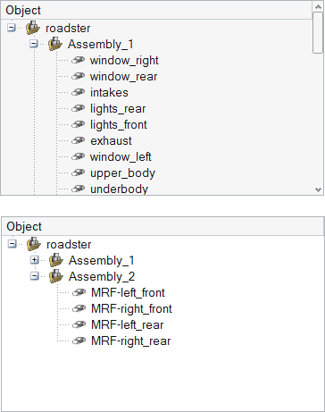
Define Wind Tunnel Dimensions
-
From the Setup group, click
Edit Tunnel.
Figure 2. 
A tunnel is generated around the model. The tunnel size is automatically set based on the best practices for vehicle simulations. -
In the Property Editor, set the Inflow speed to
30.0 m/s.
Tip: You can also double-click on the large arrow at the bottom of the wind tunnel to set the wind speed.
-
In the section labeled Boundary Layer Suction, enable the
Active checkbox, verify Inflow
is selected for Location reference, and set Distance to 10.0
m.
Any portion of the wind tunnel falling upstream of the boundary layer suction location will be treated as a slip wall. Boundary layer development will not begin until the flow passes the location that is defined in the text box.
- Optional:
Using either the Property Editor or the microdialogs in the modeling window,
modify the dimensions of the wind tunnel.
- Enter a value of 50.0 m for the length.
- Enter a value of 25.0 m for the width.
- Enter a value of 16.0 m for the height.
Figure 3. 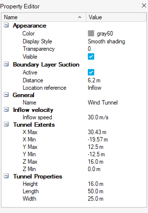
- Press Esc or right-click in empty space to exit the tool.
Identify Parts
Use the Identify Parts tool to define types of parts like wheels, heat exchangers or body panels, which require specific modeling techniques for the CFD run.
Specify the Heat Exchangers
-
To better view the heat exchangers, first Isolate relevant parts for a better
view of the heat exchangers.
-
In the Model Browser, click
 to activate the Search and Filter toolbar.
- In the text field, enter rad.
- Select all the filtered parts.
- Right-click and select Isolate from the context menu or press I.
Only the parts needed for specifying the heat exchangers are displayed.Figure 4. 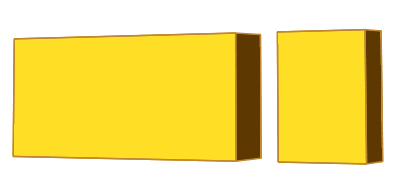
-
In the Model Browser, click
-
From the Setup group, click
Identify Parts.
Figure 5. 
-
From the secondary tool set, click Heat Exchanger.
Figure 6. 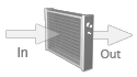
-
Specify the inflow component for the first heat exchanger.
-
Select rad_1_in in the modeling window.
Figure 7. 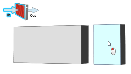
-
Select rad_1_in in the modeling window.
-
Specify the outflow component for the first heat exchanger.
-
Select rad_1_out in the modeling window.
Figure 8. 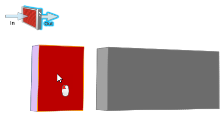
As soon as the inlet and outlet of the heat exchanger is defined, Virtual Wind Tunnel automatically identifies rad_1_frame as the connecting wall between those two surface regions. -
Select rad_1_out in the modeling window.
-
Create a second heat exchanger by clicking
 in the Heat Exchangers dialog.
-
Specify the inflow component for the second heat exchanger.
-
Select rad_2_in in the modeling window.
Figure 9. 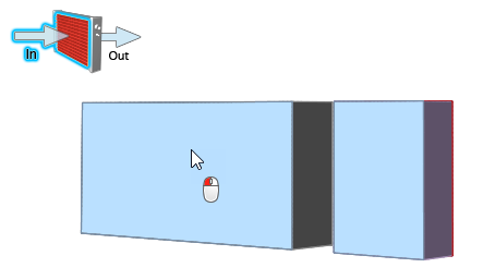
-
Select rad_2_in in the modeling window.
-
Specify the outflow component for the second heat exchanger.
-
Select rad_2_out in the modeling window.
Figure 10. 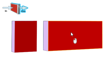
HyperMesh CFD automatically identifies rad_2_frame as the connecting wall between those two surface regions. -
Select rad_2_out in the modeling window.
- Press Esc or right-click in empty space to exit the tool.
- Delete rad from the Search and Filter text box.
- Right-click in the modeling window and select Show All Parts from the context menu or press A to return to the full model view.
Specify the Wheels
You need to select the parts forming the wheel, for example tire and rim. All other parameters like center of rotation, axis of rotation, and the angular velocity (in RPM) are computed automatically. If multiple parts are selected, HyperMesh CFD will group the parts into one or more wheels. For example, if you select the brake disc, the rim and the tire of the left front wheel, all three parts will be identified as wheel_1. If you also select the rim and the tire of the left rear wheel, those parts will be grouped into wheel_2.
-
In order to view all the parts that make up the wheels, you will need to hide
the MRF regions.
- In the Model Browser, select all the MRF parts in Assembly_2.
- Right-click and select Hide from the context menu or press H to hide the selected MRF geometry.
-
From the Setup group, click
Identify Parts.
Figure 11.
-
From the secondary tool set, click Create Wheel.
Figure 12. 
-
Select the tire, rim, hub, and brake disk of the front-left wheel.
Figure 13. 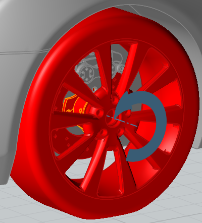
Note: You may need to rotate and zoom the model to get a better view of the wheel hub. - Repeat step 4 for the front-right wheel.
-
For the back wheels, select just the rim and tire.
Figure 14. 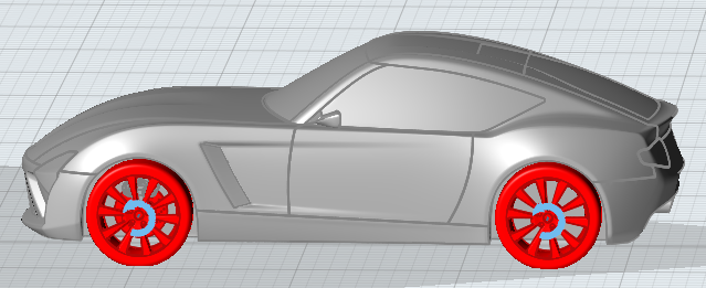
- Click on the parts now identified as wheels in the Model Browser.
- In the Property Editor, ensure that Auto Calculate is enabled for Wheel Rpm and that the Angular velocity is approximately 933 rpm.
- Press Esc or right-click in empty space to exit the tool once all the wheels have been identified.
Specify the MRF Regions
MRF regions define a volume in which the governing equations are solved in a rotating reference frame. This transformation of the equations can lead to higher accuracy for rotating bodies due the addition of centrifugal and Coriolis forces.
-
Right-click on Assembly_2 in the Model Browser and select Show from the
context menu.
The MRF geometry that was hidden in the previous step is now visible.
-
From the Setup group, click
Identify Parts.
Figure 15.
-
From the secondary tool set, click MRF.
Figure 16. 
A guide bar appears below the tool. -
Click the tire on the front-left wheel.
The entire wheel group is selected. To double-check, you can hide MRF-left_front and observe the parts you selected as the wheel in the previous step.
- On the guide bar, click MRF.
-
Select the gray disk on the front-left wheel as the MRF region.
The region is highlighted blue.
Figure 17. 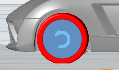
-
Click
 on the guide bar to confirm your selection.
- Click Wheel on the guide bar then select the tire on the front-right wheel.
- Click MRF then select the tire's associated MRF region.
-
Repeat the above process for the rear wheels.
Figure 18. 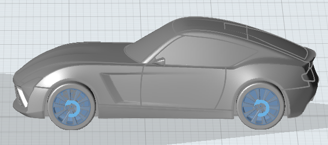
The angular velocity and center of rotation of the rotating frames are extracted from the wheel definitions.
Specify the Fan
-
Import the fan.
-
Hide the parts of the roadster model.
Tip: To show and hide a part, you can select the part and press H.
-
From the Setup group, click
Identify Parts.
Figure 19.
-
From the secondary tool set, click Create Fans.
Figure 20. 
The Fan dialog opens. - For the Selector, select the fan in the modeling window.
- For Fan Model, select OverSet.
-
In the Fan dialog, select Solid
Revolution and select the fan_volume part
in the modeling window.
Figure 21. 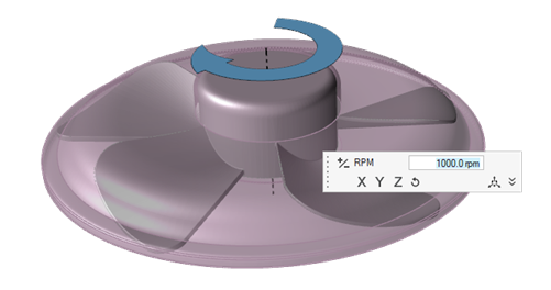
- Adjust the refinement level.
- Enable the Interface Refinement checkbox, to refine the interface of the Overset volume.
-
Adjust the Refinement Level of the interface refinement.
The Element Size will be adjusted automatically.
-
Select
 to confirm your selections and exit the dialog and
tool.
to confirm your selections and exit the dialog and
tool.
- Show the roadster model parts that were hidden in step 2.
Review Identified Parts
-
From the Setup group,
Identify Parts tool
group, click Parts.
Figure 22. 
-
In the Parts dialog, check that you identified the correct
parts as wheels and heat exchangers.
Figure 23. 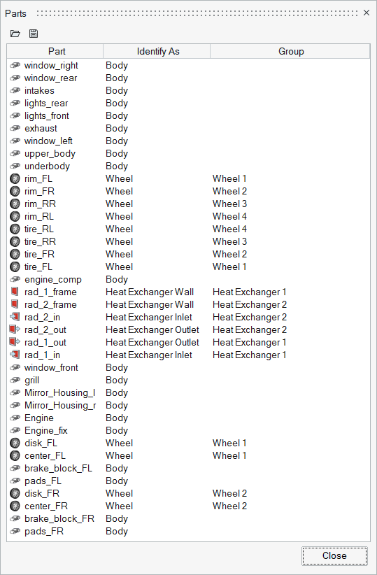
- Optional:
Click
 to export the part
definitions as an .xml template
file for use with later simulations.
to export the part
definitions as an .xml template
file for use with later simulations.
Define the Mesh Controls
Use the Mesh Controls tool to define regions with a user-defined volume element size.
Set the Far Field Element Size
-
From the Setup group, click Mesh Controls.
Figure 24. 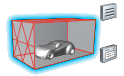
-
From the secondary tool set, click Far Field.
Figure 25. 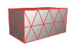
- Verify the element size value is set to 0.192 m.
Generate Box Refinement Zones Around the Body
-
From the Setup group, click Mesh Controls.
Figure 26.
-
From the secondary tool set, click the body of the Box
tool.
Figure 27. 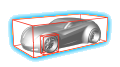
-
Select any location on the model body.
A new refinement zone is generated around the body.
-
Enter a value of 3 for Level and press
Enter.
The element size is changed to 0.0250 m.
Figure 28. 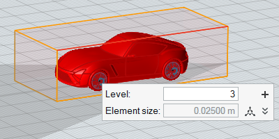
-
In the Property Editor, edit the dimensions of the
refinement zone so that the length is 5.0 m, the width is
2.0 m, the height is 2.0 m,
and X Min extent is -1.0 m.
Figure 29. 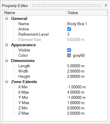
-
In the microdialog, click .
A second box refinement zone is generated.
-
Enter a value of 2 for Level and press
Enter.
The element size is changed to 0.0500 m.
- In the Property Editor, edit the dimensions of the refinement zone so that the length is 7.0 m, the width is 3.0 m, the height is 2.5 m, and the X Min extent is -1.0 m.
-
Click
once more.
A third box refinement zone is generated.
-
Enter a value of 1 for Level and press
Enter.
The element size is changed to 0.100 m.
-
In the Property Editor, edit the dimensions of the
refinement zone so that the length is 9.0 m, the width is
4.0 m, the height is 3.0 m,
and the X Min extent is -1.0 m.
Figure 30. 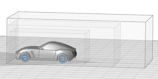
Generate Box Refinement Zones Around Parts
-
From the Setup group, click Mesh Controls.
Figure 31.
-
From the secondary tool set, click the wheel on the Box
tool.
Figure 32. 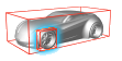
-
Select the left mirror housing in the modeling window.
A box refinement zone is generated around the part.
-
In the microdialog, enter a value of
5 for Level.
The element size is changed to 0.00625 m.
-
Modify the refinement zone's dimensions.
-
In the microdialog, click
 .
.
- Enter a value of 0.50 m for length.
- Enter a value of 0.20 m for width.
- Enter a value of 0.15 m for height.
Figure 33. 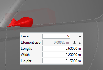
-
In the microdialog, click
- Generate a box refinement zone around the opposite mirror housing using the same dimensions for level, length, width, and height.
Generate a Body-Fitted Refinement Zone
-
From the Setup group, click Mesh Controls.
Figure 34.
-
From the secondary tool set, click the body on the Offset tool.
Figure 35. 
- Select a point on the model body.
- In the microdialog, use the drop-down menu to change the method from Distance to Layers.
-
Enter a value of 4 for Level.
The element size is changed to 0.0125 m.
-
Set the number of layers to 8.
Figure 36. 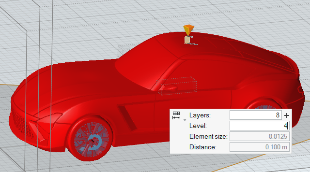
Generate Part-Fitted Refinement Zones
-
From the Setup group, click Mesh Controls.
Figure 37.
-
From the secondary tool set, click the wheel on the Offset tool.
Figure 38. 
- Hold Ctrl and left-click on all four sets of tires and rims in the modeling window.
- In the microdialog, use the drop-down menu to change the method from Distance to Layers.
-
Enter a value of 5 for Level.
The element size is changed to 0.00625 m.
-
Set the number of layers to 5.
Figure 39. 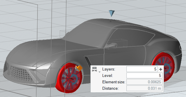
-
Click .
A second part-fitted refinement zone is created around the four wheels.
-
Enter a value of 4 for Level.
The element size is changed to 0.0125 m.
-
Set the number of layers to 10.
Figure 40. 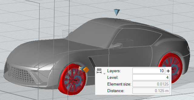
- Press Esc or right-click in empty space to exit the tool.
Review Mesh Controls
-
From the Setup group,
Mesh Controls tool
group, click Zones.
Figure 41. 
-
Double-check the refinement zones and make sure they match what's displayed in
Figure 42.
Figure 42. 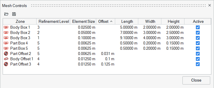
- Optional:
Click to export the mesh control
definitions as an .xml template
file for use with later simulations.
- Click Close to exit the dialog.
Define the Belt System
-
From the Setup group, click
Belt System.
Figure 43. 
By default, five patches are created on the wind tunnel ground for modeling the belt system.Figure 44. 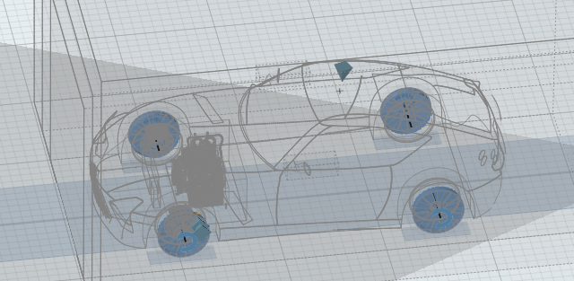
- Accept the default parameters for the belts.
Define the Output Frequency
-
From the Output group, click
General Output.
Figure 45. 
The Output Controls dialog opens. -
In the Output Controls dialog, enter
100 for the output frequency.
This tells the solver to write simulation results every 100 iterations.
Submit Job
-
From the Run group, click
Run.
Figure 46. 
- In the Write to ultraFluidX dialog, enter a name for the run.
- Click Results to view more options.
-
Accept all other default parameters.
Figure 47. 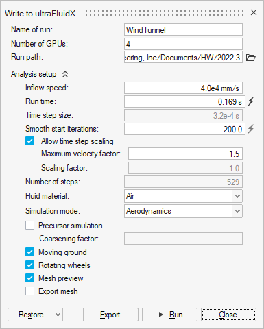
-
Click Run.
If you are running HyperMesh CFD on a Linux system with a supported GPU, no further configuration steps are necessary. If you are running HyperMesh CFD on a Windows system, you'll need to have a Linux installation of ultraFluidX available for running the solver. To run the solver from Windows:
Plot Aero Coefficients
-
From the Run group, click
Plot Aero Coefficients.
Figure 48. 
-
Browse to the path you defined as the default run directory and select
uFX_coefficients_Inst.txt .
A graph of the instantaneous lift, drag, and side force coefficients is displayed.
Figure 49. 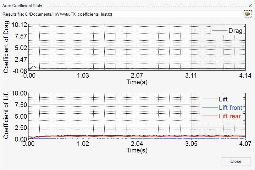
-
Browse to the default directory once more and select
uFX_coefficients_Avg.txt.
A graph of the time averaged lift, drag, and side force coefficients is displayed.
Figure 50. 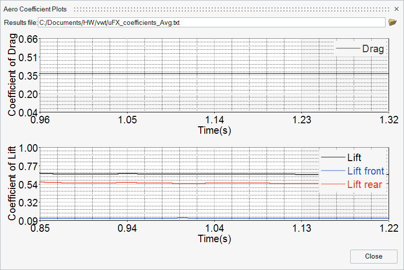
-
Middle-mouse scroll to zoom in on points of interest in the plot.
Note: Other plots, including coefficients for each part individually are also available in the output directory.