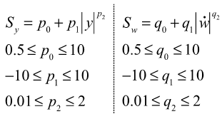
These factors are used to represent friction in the bushing material and also other
effects such as viscoelasticity.
The overall scale factor is defined on the left for stiffness and on the right for
damping as follows:
The following plot shows the behavior of the scaling function
S
y
MathType@MTEF@5@5@+=
feaagKart1ev2aaatCvAUfeBSjuyZL2yd9gzLbvyNv2CaerbuLwBLn
hiov2DGi1BTfMBaeXatLxBI9gBaerbd9wDYLwzYbItLDharqqtubsr
4rNCHbGeaGqiVu0Je9sqqrpepC0xbbL8F4rqqrFfpeea0xe9Lq=Jc9
vqaqpepm0xbba9pwe9Q8fs0=yqaqpepae9pg0FirpepeKkFr0xfr=x
fr=xb9adbaqaaeGaciGaaiaabeqaamaabaabaaGcbaGaam4uamaaBa
aaleaacaWG5baabeaaaaa@37F8@
|
y
|
MathType@MTEF@5@5@+=
feaagKart1ev2aaatCvAUfeBSjuyZL2yd9gzLbvyNv2CaerbuLwBLn
hiov2DGi1BTfMBaeXatLxBI9gBaerbd9wDYLwzYbItLDharqqtubsr
4rNCHbGeaGqiVu0Je9sqqrpepC0xbbL8F4rqqrFfpeea0xe9Lq=Jc9
vqaqpepm0xbba9pwe9Q8fs0=yqaqpepae9pg0FirpepeKkFr0xfr=x
fr=xb9adbaqaaeGaciGaaiaabeqaamaabaabaaGcbaWaaqWaaeaaca
WG5baacaGLhWUaayjcSdaaaa@3A16@
p
2
MathType@MTEF@5@5@+=
feaagKart1ev2aaatCvAUfeBSjuyZL2yd9gzLbvyNv2CaerbuLwBLn
hiov2DGi1BTfMBaeXatLxBI9gBaerbd9wDYLwzYbItLDharqqtubsr
4rNCHbGeaGqiVu0Je9sqqrpepC0xbbL8F4rqqrFfpeea0xe9Lq=Jc9
vqaqpepm0xbba9pwe9Q8fs0=yqaqpepae9pg0FirpepeKkFr0xfr=x
fr=xb9adbaqaaeGaciGaaiaabeqaamaabaabaaGcbaGaamiCamaaBa
aaleaacaaIYaaabeaaaaa@37D3@
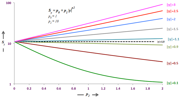
Figure 1 . The functional form of
S
y
MathType@MTEF@5@5@+=
feaagKart1ev2aaatCvAUfeBSjuyZL2yd9gzLbvyNv2CaerbuLwBLn
hiov2DGi1BTfMBaeXatLxBI9gBaerbd9wDYLwzYbItLDharqqtubsr
4rNCHbGeaGqiVu0Je9sqqrpepC0xbbL8F4rqqrFfpeea0xe9Lq=Jc9
vqaqpepm0xbba9pwe9Q8fs0=yqaqpepae9pg0FirpepeKkFr0xfr=x
fr=xb9adbaqaaeGaciGaaiaabeqaamaabaabaaGcbaGaam4uamaaBa
aaleaacaWG5baabeaaaaa@37F8@
is selected as it easily represents a variety of
shapes with very few parameters.
Note:
S
y
MathType@MTEF@5@5@+=
feaagKart1ev2aaatCvAUfeBSjuyZL2yd9gzLbvyNv2CaerbuLwBLn
hiov2DGi1BTfMBaeXatLxBI9gBaerbd9wDYLwzYbItLDharqqtubsr
4rNCHbGeaGqiVu0Je9sqqrpepC0xbbL8F4rqqrFfpeea0xe9Lq=Jc9
vqaqpepm0xbba9pwe9Q8fs0=yqaqpepae9pg0FirpepeKkFr0xfr=x
fr=xb9adbaqaaeGaciGaaiaabeqaamaabaabaaGcbaGaam4uamaaBa
aaleaacaWG5baabeaaaaa@37F8@
and
S
w
MathType@MTEF@5@5@+=
feaagKart1ev2aaatCvAUfeBSjuyZL2yd9gzLbvyNv2CaerbuLwBLn
hiov2DGi1BTfMBaeXatLxBI9gBaerbd9wDYLwzYbItLDharqqtubsr
4rNCHbGeaGqiVu0Je9sqqrpepC0xbbL8F4rqqrFfpeea0xe9Lq=Jc9
vqaqpepm0xbba9pwe9Q8fs0=yqaqpepae9pg0FirpepeKkFr0xfr=x
fr=xb9adbaqaaeGaciGaaiaabeqaamaabaabaaGcbaGaam4uamaaBa
aaleaacaWG3baabeaaaaa@37F6@
are primarily responsible for capturing the
dependency of the dynamic stiffness and loss angle on the amplitude of the
input.
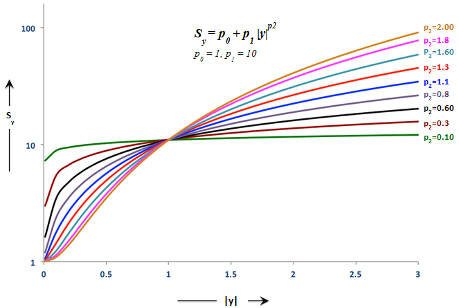
The next figure shows the same data as the figure above, except
|
y
|
MathType@MTEF@5@5@+=
feaagKart1ev2aaatCvAUfeBSjuyZL2yd9gzLbvyNv2CaerbuLwBLn
hiov2DGi1BTfMBaeXatLxBI9gBaerbd9wDYLwzYbItLDharqqtubsr
4rNCHbGeaGqiVu0Je9sqqrpepC0xbbL8F4rqqrFfpeea0xe9Lq=Jc9
vqaqpepm0xbba9pwe9Q8fs0=yqaqpepae9pg0FirpepeKkFr0xfr=x
fr=xb9adbaqaaeGaciGaaiaabeqaamaabaabaaGcbaWaaqWaaeaaca
WG5baacaGLhWUaayjcSdaaaa@3A16@
p
2
MathType@MTEF@5@5@+=
feaagKart1ev2aaatCvAUfeBSjuyZL2yd9gzLbvyNv2CaerbuLwBLn
hiov2DGi1BTfMBaeXatLxBI9gBaerbd9wDYLwzYbItLDharqqtubsr
4rNCHbGeaGqiVu0Je9sqqrpepC0xbbL8F4rqqrFfpeea0xe9Lq=Jc9
vqaqpepm0xbba9pwe9Q8fs0=yqaqpepae9pg0FirpepeKkFr0xfr=x
fr=xb9adbaqaaeGaciGaaiaabeqaamaabaabaaGcbaGaamiCamaaBa
aaleaacaaIYaaabeaaaaa@37D3@
Figure 2 .