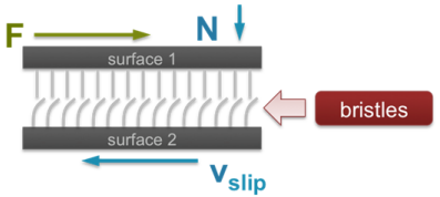
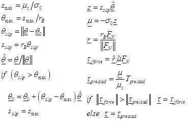
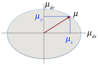
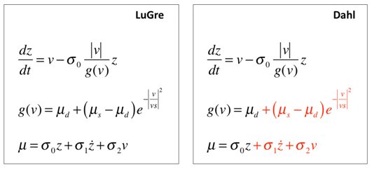
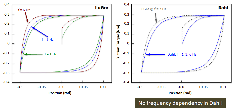
Friction Formulation This section provides information about the LuGre and Dahl formulations for friction. LuGre Model The LuGre model, which supports both stiction and dynamic friction, is implemented. In the LuGre formulation, a bristle model is used to idealize friction. When a tangential motion arises between the surfaces, the bristles deflect like springs. If the deflection is sufficiently large, the bristles start to slip. A bristle model is used to idealize the friction between two mating surfaces. The slip velocity between the mating surfaces, V s l i p MathType@MTEF@5@5@+= feaagKart1ev2aaatCvAUfeBSjuyZL2yd9gzLbvyNv2CaerbuLwBLn hiov2DGi1BTfMBaeXatLxBI9gBaerbd9wDYLwzYbItLDharqqtubsr 4rNCHbGeaGqiVu0Je9sqqrpepC0xbbL8F4rqqrFfpeea0xe9Lq=Jc9 vqaqpepm0xbba9pwe9Q8fs0=yqaqpepae9pg0FirpepeKkFr0xfr=x fr=xb9adbaqaaeGaciGaaiaabeqaamaabaabaaGcbaGaamOvamaaBa aaleaacaWGZbGaamiBaiaadMgacaWGWbaabeaaaaa@3AC9@ , determines the average bristle deflection for a steady state motion. It is lower at low velocities, which implies that the steady state deflection decreases with increasing velocity. The figure below depicts the bristle model:Figure 1. The LuGre model represents several different effects: The effect of the mating surfaces being pushed apart by lubricant. The Stribeck effect at very low speed. When partial fluid lubrication exists, contact between the surfaces decreases and thus friction decreases exponentially from stiction. Rate dependent friction phenomena such as varying break-away force and frictional lag. Static friction between two surfaces. Define the following quantities: r b MathType@MTEF@5@5@+= feaagKart1ev2aaatCvAUfeBSjuyZL2yd9gzLbvyNv2CaerbuLwBLn hiov2DGi1BTfMBaeXatLxBI9gBaerbd9wDYLwzYbItLDharqqtubsr 4rNCHbGeaGqiVu0Je9sqqrpepC0xbbL8F4rqqrFfpeea0xe9Lq=Jc9 vqaqpepm0xbba9pwe9Q8fs0=yqaqpepae9pg0FirpepeKkFr0xfr=x fr=xb9adbaqaaeGaciGaaiaabeqaamaabaabaaGcbaGaamOCaiaadk gaaaa@37D4@ Ball radius F N MathType@MTEF@5@5@+= feaagKart1ev2aaatCvAUfeBSjuyZL2yd9gzLbvyNv2CaerbuLwBLn hiov2DGi1BTfMBaeXatLxBI9gBaerbd9wDYLwzYbItLDharqqtubsr 4rNCHbGeaGqiVu0Je9sqqrpepC0xbbL8F4rqqrFfpeea0xe9Lq=Jc9 vqaqpepm0xbba9pwe9Q8fs0=yqaqpepae9pg0FirpepeKkFr0xfr=x fr=xb9adbaqaaeGaciGaaiaabeqaamaabaabaaGcbaGaamOramaaBa aaleaacaWGobaabeaaaaa@37C0@ Normal force between a pair of surfaces. μ s MathType@MTEF@5@5@+= feaagKart1ev2aaatCvAUfeBSjuyZL2yd9gzLbvyNv2CaerbuLwBLn hiov2DGi1BTfMBaeXatLxBI9gBaerbd9wDYLwzYbItLDharqqtubsr 4rNCHbGeaGqiVu0Je9sqqrpepC0xbbL8F4rqqrFfpeea0xe9Lq=Jc9 vqaqpepm0xbba9pwe9Q8fs0=yqaqpepae9pg0FirpepeKkFr0xfr=x fr=xb9adbaqaaeGaciGaaiaabeqaamaabaabaaGcbaGaeqiVd02aaS baaSqaaiaadohaaeqaaaaa@38D0@ Coefficient of static friction. μ d MathType@MTEF@5@5@+= feaagKart1ev2aaatCvAUfeBSjuyZL2yd9gzLbvyNv2CaerbuLwBLn hiov2DGi1BTfMBaeXatLxBI9gBaerbd9wDYLwzYbItLDharqqtubsr 4rNCHbGeaGqiVu0Je9sqqrpepC0xbbL8F4rqqrFfpeea0xe9Lq=Jc9 vqaqpepm0xbba9pwe9Q8fs0=yqaqpepae9pg0FirpepeKkFr0xfr=x fr=xb9adbaqaaeGaciGaaiaabeqaamaabaabaaGcbaGaeqiVd02aaS baaSqaaiaadsgaaeqaaaaa@38C1@ Coefficient of dynamic friction (µd ≤ µs). T MathType@MTEF@5@5@+= feaagKart1ev2aaatCvAUfeBSjuyZL2yd9gzLbvyNv2CaerbuLwBLn hiov2DGi1BTfMBaeXatLxBI9gBaerbd9wDYLwzYbItLDharqqtubsr 4rNCHbGeaGqiVu0Je9sqqrpepC0xbbL8F4rqqrFfpeea0xe9Lq=Jc9 vqaqpepm0xbba9pwe9Q8fs0=yqaqpepae9pg0FirpepeKkFr0xfr=x fr=xb9adbaqaaeGaciGaaiaabeqaamaabaabaaGcbaGaamivaaaa@36CF@ True friction torque between the surfaces. σ 0 , σ 1 , σ 2 , v s MathType@MTEF@5@5@+= feaagKart1ev2aaatCvAUfeBSjuyZL2yd9gzLbvyNv2CaerbuLwBLn hiov2DGi1BTfMBaeXatLxBI9gBaerbd9wDYLwzYbItLDharqqtubsr 4rNCHbGeaGqiVu0Je9sqqrpepC0xbbL8F4rqqrFfpeea0xe9Lq=Jc9 vqaqpepm0xbba9pwe9Q8fs0=yqaqpepae9pg0FirpepeKkFr0xfr=x fr=xb9adbaqaaeGaciGaaiaabeqaamaabaabaaGcbaGaeq4Wdm3aaS baaSqaaiaaicdaaeqaaOGaaiilaiaaysW7cqaHdpWCdaWgaaWcbaGa aGymaaqabaGccaGGSaGaaGjbVlabeo8aZnaaBaaaleaacaaIYaaabe aakiaacYcacaaMe8UaamODamaaBaaaleaacaWGZbaabeaaaaa@46E8@ Constants associated with the LuGre model. Assuming contact on a spherical surface, the friction force is a 2-dimensional quantity in the friction plane, but a 3-dimensional quantity in the I-Marker coordinate system. Joint friction is calculated using the algorithm shown next: Quantity Formula Angular slip velocity ω _ = [ ω x ω y ω z ] T ; ω m = ‖ ω _ ‖ MathType@MTEF@5@5@+= feaagKart1ev2aaatCvAUfeBSjuyZL2yd9gzLbvyNv2CaerbuLwBLn hiov2DGi1BTfMBaeXatLxBI9gBaerbd9wDYLwzYbItLDharqqtubsr 4rNCHbGeaGqiVu0Je9sqqrpepC0xbbL8F4rqqrFfpeea0xe9Lq=Jc9 vqaqpepm0xbba9pwe9Q8fs0=yqaqpepae9pg0FirpepeKkFr0xfr=x fr=xb9adbaqaaeGaciGaaiaabeqaamaabaabaaGcbaGafqyYdCNba0 bacqGH9aqpdaWadaqaamaaBaaaleaacqaHjpWDdaWgaaadbaGaamiE aaqabaWccaaMe8UaaGjbVlaaysW7cqaHjpWDdaWgaaadbaGaamyEaa qabaWccaaMe8UaaGjbVlaaysW7cqaHjpWDdaWgaaadbaGaamOEaaqa baaaleqaaaGccaGLBbGaayzxaaWaaWbaaSqabeaacaWGubaaaOGaai 4oaiaaysW7cqaHjpWDdaWgaaWcbaGaamyBaaqabaGccqGH9aqpdaqb daqaaiqbeM8a3zaaDaaacaGLjWUaayPcSdaaaa@59DB@ Bristle states z _ = [ z x z y z z ] T MathType@MTEF@5@5@+= feaagKart1ev2aaatCvAUfeBSjuyZL2yd9gzLbvyNv2CaerbuLwBLn hiov2DGi1BTfMBaeXatLxBI9gBaerbd9wDYLwzYbItLDharqqtubsr 4rNCHbGeaGqiVu0Je9sqqrpepC0xbbL8F4rqqrFfpeea0xe9Lq=Jc9 vqaqpepm0xbba9pwe9Q8fs0=yqaqpepae9pg0FirpepeKkFr0xfr=x fr=xb9adbaqaaeGaciGaaiaabeqaamaabaabaaGcbaGabmOEayaaDa Gaeyypa0ZaamWaaeaadaWgaaWcbaGaamOEamaaBaaameaacaWG4baa beaaliaaysW7caaMe8UaaGjbVlaadQhadaWgaaadbaGaamyEaaqaba WccaaMe8UaaGjbVlaaysW7caWG6bWaaSbaaWqaaiaadQhaaeqaaaWc beaaaOGaay5waiaaw2faamaaCaaaleqabaGaamivaaaaaaa@4B3A@ Stiction to dynamic friction transition function g ( ω m ) = μ d + ( μ s − μ d ) e − ( r B ⋅ ω m / v s ) 2 MathType@MTEF@5@5@+= feaagKart1ev2aaatCvAUfeBSjuyZL2yd9gzLbvyNv2CaerbuLwBLn hiov2DGi1BTfMBaeXatLxBI9gBaerbd9wDYLwzYbItLDharqqtubsr 4rNCHbGeaGqiVu0Je9sqqrpepC0xbbL8F4rqqrFfpeea0xe9Lq=Jc9 vqaqpepm0xbba9pwe9Q8fs0=yqaqpepae9pg0FirpepeKkFr0xfr=x fr=xb9adbaqaaeGaciGaaiaabeqaamaabaabaaGcbaGaam4zamaabm aabaGaeqyYdC3aaSbaaSqaaiaad2gaaeqaaaGccaGLOaGaayzkaaGa eyypa0JaeqiVd02aaSbaaSqaaiaadsgaaeqaaOGaey4kaSYaaeWaae aacqaH8oqBdaWgaaWcbaGaam4CaaqabaGccqGHsislcqaH8oqBdaWg aaWcbaGaamizaaqabaaakiaawIcacaGLPaaacaWGLbWaaWbaaSqabe aacqGHsisldaqadaqaamaalyaabaGaamOCamaaBaaameaacaWGcbaa beaaliabgwSixlabeM8a3naaBaaameaacaWGTbaabeaaaSqaaiaadA hadaWgaaadbaGaam4CaaqabaaaaaWccaGLOaGaayzkaaWaaWbaaWqa beaacaaIYaaaaaaaaaa@563B@ Coupling function λ ( ω m ) = r B ω m μ d 2 g ( ω m ) MathType@MTEF@5@5@+= feaagKart1ev2aaatCvAUfeBSjuyZL2yd9gzLbvyNv2CaerbuLwBLn hiov2DGi1BTfMBaeXatLxBI9gBaerbd9wDYLwzYbItLDharqqtubsr 4rNCHbGeaGqiVu0Je9sqqrpepC0xbbL8F4rqqrFfpeea0xe9Lq=Jc9 vqaqpepm0xbba9pwe9Q8fs0=yqaqpepae9pg0FirpepeKkFr0xfr=x fr=xb9adbaqaaeGaciGaaiaabeqaamaabaabaaGcbaGaeq4UdW2aae WaaeaacqaHjpWDdaWgaaWcbaGaamyBaaqabaaakiaawIcacaGLPaaa cqGH9aqpdaWcaaqaaiaadkhadaWgaaWcbaGaamOqaaqabaGccqaHjp WDdaWgaaWcbaGaamyBaaqabaGccqaH8oqBdaqhaaWcbaGaamizaaqa aiaaikdaaaaakeaacaWGNbWaaeWaaeaacqaHjpWDdaWgaaWcbaGaam yBaaqabaaakiaawIcacaGLPaaaaaaaaa@4B23@ Rate dependence function C 0 ( ω m ) = λ ( ω m ) σ 0 μ d 2 = r B ω m σ 0 g ( ω m ) MathType@MTEF@5@5@+= feaagKart1ev2aaatCvAUfeBSjuyZL2yd9gzLbvyNv2CaerbuLwBLn hiov2DGi1BTfMBaeXatLxBI9gBaerbd9wDYLwzYbItLDharqqtubsr 4rNCHbGeaGqiVu0Je9sqqrpepC0xbbL8F4rqqrFfpeea0xe9Lq=Jc9 vqaqpepm0xbba9pwe9Q8fs0=yqaqpepae9pg0FirpepeKkFr0xfr=x fr=xb9adbaqaaeGaciGaaiaabeqaamaabaabaaGcbaGaam4qamaaBa aaleaacaaIWaaabeaakmaabmaabaGaeqyYdC3aaSbaaSqaaiaad2ga aeqaaaGccaGLOaGaayzkaaGaeyypa0ZaaSaaaeaacqaH7oaBdaqada qaaiabeM8a3naaBaaaleaacaWGTbaabeaaaOGaayjkaiaawMcaaiab eo8aZnaaBaaaleaacaaIWaaabeaaaOqaaiabeY7aTnaaDaaaleaaca WGKbaabaGaaGOmaaaaaaGccqGH9aqpdaWcaaqaaiaadkhadaWgaaWc baGaamOqaaqabaGccqaHjpWDdaWgaaWcbaGaamyBaaqabaGccqaHdp WCdaWgaaWcbaGaaGimaaqabaaakeaacaWGNbWaaeWaaeaacqaHjpWD daWgaaWcbaGaamyBaaqabaaakiaawIcacaGLPaaaaaaaaa@57D5@ Model for dynamic simulation z _ = r B ω _ − C 0 z _ MathType@MTEF@5@5@+= feaagKart1ev2aaatCvAUfeBSjuyZL2yd9gzLbvyNv2CaerbuLwBLn hiov2DGi1BTfMBaeXatLxBI9gBaerbd9wDYLwzYbItLDharqqtubsr 4rNCHbGeaGqiVu0Je9sqqrpepC0xbbL8F4rqqrFfpeea0xe9Lq=Jc9 vqaqpepm0xbba9pwe9Q8fs0=yqaqpepae9pg0FirpepeKkFr0xfr=x fr=xb9adbaqaaeGaciGaaiaabeqaamaabaabaaGcbaGabmOEayaaDa Gaeyypa0JaamOCamaaBaaaleaacaWGcbaabeaakiqbeM8a3zaaDaGa eyOeI0Iaam4qamaaBaaaleaacaaIWaaabeaakiqadQhagaqhaaaa@3FCC@ μ = − ( σ 0 z _ + σ 1 z _ + σ 2 r ω _ ) MathType@MTEF@5@5@+= feaagKart1ev2aaatCvAUfeBSjuyZL2yd9gzLbvyNv2CaerbuLwBLn hiov2DGi1BTfMBaeXatLxBI9gBaerbd9wDYLwzYbItLDharqqtubsr 4rNCHbGeaGqiVu0Je9sqqrpepC0xbbL8F4rqqrFfpeea0xe9Lq=Jc9 vqaqpepm0xbba9pwe9Q8fs0=yqaqpepae9pg0FirpepeKkFr0xfr=x fr=xb9adbaqaaeGaciGaaiaabeqaamaabaabaaGcbaGaeqiVd0Maey ypa0JaeyOeI0YaaeWaaeaacqaHdpWCdaWgaaWcbaGaaGimaaqabaGc ceWG6bGba0bacqGHRaWkcqaHdpWCdaWgaaWcbaGaaGymaaqabaGcce WG6bGba0bacqGHRaWkcqaHdpWCdaWgaaWcbaGaaGOmaaqabaGccaWG YbGafqyYdCNba0baaiaawIcacaGLPaaaaaa@4A36@ r _ = r B F _ N / ‖ F _ N ‖ MathType@MTEF@5@5@+= feaagKart1ev2aaatCvAUfeBSjuyZL2yd9gzLbvyNv2CaerbuLwBLn hiov2DGi1BTfMBaeXatLxBI9gBaerbd9wDYLwzYbItLDharqqtubsr 4rNCHbGeaGqiVu0Je9sqqrpepC0xbbL8F4rqqrFfpeea0xe9Lq=Jc9 vqaqpepm0xbba9pwe9Q8fs0=yqaqpepae9pg0FirpepeKkFr0xfr=x fr=xb9adbaqaaeGaciGaaiaabeqaamaabaabaaGcbaGabmOCayaaDa Gaeyypa0ZaaSGbaeaacaWGYbWaaSbaaSqaaiaadkeaaeqaaOGabmOr ayaaDaWaaSbaaSqaaiaad6eaaeqaaaGcbaWaauWaaeaaceWGgbGba0 badaWgaaWcbaGaamOtaaqabaaakiaawMa7caGLkWoaaaaaaa@4138@ τ _ j f o r c e = r ˜ _ μ ˜ _ F _ N MathType@MTEF@5@5@+= feaagKart1ev2aaatCvAUfeBSjuyZL2yd9gzLbvyNv2CaerbuLwBLn hiov2DGi1BTfMBaeXatLxBI9gBaerbd9wDYLwzYbItLDharqqtubsr 4rNCHbGeaGqiVu0Je9sqqrpepC0xbbL8F4rqqrFfpeea0xe9Lq=Jc9 vqaqpepm0xbba9pwe9Q8fs0=yqaqpepae9pg0FirpepeKkFr0xfr=x fr=xb9adbaqaaeGaciGaaiaabeqaamaabaabaaGcbaGafqiXdqNba0 badaWgaaWcbaGaamOAaiaadAgacaWGVbGaamOCaiaadogacaWGLbaa beaakiabg2da9iqadkhagaacgaqhaiqbeY7aTzaaiyaaDaGabmOray aaDaWaaSbaaSqaaiaad6eaaeqaaaaa@43B1@ τ _ p r e l o a d = ( μ _ / μ s ) T p r e l o a d MathType@MTEF@5@5@+= feaagKart1ev2aaatCvAUfeBSjuyZL2yd9gzLbvyNv2CaerbuLwBLn hiov2DGi1BTfMBaeXatLxBI9gBaerbd9wDYLwzYbItLDharqqtubsr 4rNCHbGeaGqiVu0Je9sqqrpepC0xbbL8F4rqqrFfpeea0xe9Lq=Jc9 vqaqpepm0xbba9pwe9Q8fs0=yqaqpepae9pg0FirpepeKkFr0xfr=x fr=xb9adbaqaaeGaciGaaiaabeqaamaabaabaaGcbaGafqiXdqNba0 badaWgaaWcbaGaamiCaiaadkhacaWGLbGaamiBaiaad+gacaWGHbGa amizaaqabaGccqGH9aqpdaqadaqaamaalyaabaGafqiVd0Mba0baae aacqaH8oqBdaWgaaWcbaGaam4CaaqabaaaaaGccaGLOaGaayzkaaGa amivamaaBaaaleaacaWGWbGaamOCaiaadwgacaWGSbGaam4Baiaadg gacaWGKbaabeaaaaa@4D91@ f ‖ τ _ j f o r c e ‖ > ‖ τ _ p r e l o a d ‖ τ _ = τ _ j f o r c e MathType@MTEF@5@5@+= feaagKart1ev2aaatCvAUfeBSjuyZL2yd9gzLbvyNv2CaerbuLwBLn hiov2DGi1BTfMBaeXatLxBI9gBaerbd9wDYLwzYbItLDharqqtubsr 4rNCHbGeaGqiVu0Je9sqqrpepC0xbbL8F4rqqrFfpeea0xe9Lq=Jc9 vqaqpepm0xbba9pwe9Q8fs0=yqaqpepae9pg0FirpepeKkFr0xfr=x fr=xb9adbaqaaeGaciGaaiaabeqaamaabaabaaGcbaGaamOzaiaays W7daqbdaqaaiqbes8a0zaaDaWaaSbaaSqaaiaadQgacaWGMbGaam4B aiaadkhacaWGJbGaamyzaaqabaaakiaawMa7caGLkWoacqGH+aGpda qbdaqaaiqbes8a0zaaDaWaaSbaaSqaaiaadchacaWGYbGaamyzaiaa dYgacaWGVbGaamyyaiaadsgaaeqaaaGccaGLjWUaayPcSdGaaGjbVl aaysW7c0aJasiXdqNbiWiGDaGaeyypa0JafqiXdqNba0badaWgaaWc baGaamOAaiaadAgacaWGVbGaamOCaiaadogacaWGLbaabeaaaaa@6000@ e l s e τ _ = τ _ p r e l o a d MathType@MTEF@5@5@+= feaagKart1ev2aaatCvAUfeBSjuyZL2yd9gzLbvyNv2CaerbuLwBLn hiov2DGi1BTfMBaeXatLxBI9gBaerbd9wDYLwzYbItLDharqqtubsr 4rNCHbGeaGqiVu0Je9sqqrpepC0xbbL8F4rqqrFfpeea0xe9Lq=Jc9 vqaqpepm0xbba9pwe9Q8fs0=yqaqpepae9pg0FirpepeKkFr0xfr=x fr=xb9adbaqaaeGaciGaaiaabeqaamaabaabaaGcbaGaamyzaiaadY gacaWGZbGaamyzaiaaysW7cuaHepaDgaqhaiabg2da9iqbes8a0zaa DaWaaSbaaSqaaiaadchacaWGYbGaamyzaiaadYgacaWGVbGaamyyai aadsgaaeqaaaaa@46CE@ Model for static simulation The LuGre model supports the notion of a friction ellipse. The term in the above equations, λ ( ω r ) MathType@MTEF@5@5@+= feaagKart1ev2aaatCvAUfeBSjuyZL2yd9gzLbvyNv2CaerbuLwBLn hiov2DGi1BTfMBaeXatLxBI9gBaerbd9wDYLwzYbItLDharqqtubsr 4rNCHbGeaGqiVu0Je9sqqrpepC0xbbL8F4rqqrFfpeea0xe9Lq=Jc9 vqaqpepm0xbba9pwe9Q8fs0=yqaqpepae9pg0FirpepeKkFr0xfr=x fr=xb9adbaqaaeGaciGaaiaabeqaamaabaabaaGcbaGaeq4UdW2aae WaaeaacqaHjpWDdaWgaaWcbaGaamOCaaqabaaakiaawIcacaGLPaaa aaa@3C2D@ , represents the coupling effect between the friction forces in two orthogonal directions in the friction plane. This coupling effect leads to the familiar friction ellipse that defines the limiting forces when sliding is seen in both orthogonal directions, as shown in the figure below:Figure 2. Dahl Model as a Subset of the LuGre Model The Dahl model of friction can be obtained from the LuGre model simply by setting the parameters σ 1 = o , σ 2 = 0 MathType@MTEF@5@5@+= feaagKart1ev2aaatCvAUfeBSjuyZL2yd9gzLbvyNv2CaerbuLwBLn hiov2DGi1BTfMBaeXatLxBI9gBaerbd9wDYLwzYbItLDharqqtubsr 4rNCHbGeaGqiVu0Je9sqqrpepC0xbbL8F4rqqrFfpeea0xe9Lq=Jc9 vqaqpepm0xbba9pwe9Q8fs0=yqaqpepae9pg0FirpepeKkFr0xfr=x fr=xb9adbaqaaeGaciGaaiaabeqaamaabaabaaGcbaGaeq4Wdm3aaS baaSqaaiaaigdaaeqaaOGaeyypa0Jaam4BaiaacYcacaaMe8Uaeq4W dm3aaSbaaSqaaiaaikdaaeqaaOGaeyypa0JaaGimaaaa@4156@ and μ s = μ d MathType@MTEF@5@5@+= feaagKart1ev2aaatCvAUfeBSjuyZL2yd9gzLbvyNv2CaerbuLwBLn hiov2DGi1BTfMBaeXatLxBI9gBaerbd9wDYLwzYbItLDharqqtubsr 4rNCHbGeaGqiVu0Je9sqqrpepC0xbbL8F4rqqrFfpeea0xe9Lq=Jc9 vqaqpepm0xbba9pwe9Q8fs0=yqaqpepae9pg0FirpepeKkFr0xfr=x fr=xb9adbaqaaeGaciGaaiaabeqaamaabaabaaGcbaGaeqiVd02aaS baaSqaaiaadohaaeqaaOGaeyypa0JaeqiVd02aaSbaaSqaaiaadsga aeqaaaaa@3CAB@ , as explained in the figure below. The Dahl model does not use the terms shown in red.Figure 3. Comparison Between the Dahl and LuGre Models The Dahl model requires fewer parameters. In the absence of experimental data, one should use the Dahl model. However, the Dahl does not capture many of the effects of the LuGre model. The Dahl model does not support: Stribeck effect (also known as the stick-slip effect) Static Friction > Dynamic Friction Bristle damping Memory-less damping (viscous damping) Rate dependency (such as dependency of friction force on frequency of input)! Rate dependency is an important property and is illustrated in the figure below:Figure 4. The curves in the figure represent the hysteresis loop in the friction models that cause energy dissipation. Notice that the LuGre model (left) is sensitive to the frequency of the input. In contrast the Dahl model (right) shows no change in its response even when the frequency of the inputs change.