MIT and the Fitting Process
- Fitting test data from frequency- and amplitude-dependent bushings to empirical models of bushings.
- Running a simulation using fitted parameters with an empirical model.
Fitting a Bushing Model
- Input
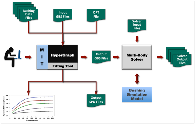
- Fitting begins with Bushing Data files. These are Input System Property
Data files in ASCII format, also known as
Input SPD files. Once you have the required .spd
files, you do three things in the MIT:
- Select a bushing model.
- Define the initial guesses of parameters for the built-in optimizer that does the fitting. The initial guesses are stored in General Bushing System files in ASCII format, known as Input GPD files.
- Specify settings in a third ASCII text file, known as the OPT file.
- Analysis
-
- The MIT interacts with an embedded Fitting Tool, which contains models for frequency- and amplitude-dependent bushings and hydromounts. The fitting tool also includes optimization algorithms to rationally change the model coefficients to fit the experimental data.
- Once the fitting is complete and a set of model parameters is determined, the fitting tool communicates the fitted model parameters back to the MIT.
- Output
-
- The fitting tool generates three key outputs: an output SPD file, an output GBS file and a Fit Report.
- The output .spd file contains the dynamic-stiffness and loss-angle behavior of the fitted model. The MIT plots the data in the input .spd file, which contains data from the physical test, and the output .spd file, which includes the data for the analytical model behavior to help you gauge the quality of the fit.
- The output .gbs file contains the fitted model parameters. This file can be used in a downstream simulation.
- The Fit Report is a PDF that contains a summary of the fit process.
Simulations
- Modeling
- Create your model using a multibody pre-processor such as MotionView. MotionView includes a comprehensive user interface for instantiating frequency- and amplitude-dependent bushings. Within MotionView, you can create a full vehicle model, and then run an analysis using MotionSolve.
- Analysis
- Perform an analysis using a multibody solver such as MotionSolve.
- Output
- The analysis of the model generates various solver output files. You can review these files with post-processors such as HyperGraph and HyperView to understand the behavior of the model.
Files Summary
| File | Extension | Format | Purpose |
|---|---|---|---|
| Input GBS | .gbs | TeimOrbit | Stores the initial guesses of parameters and settings that are used for fitting model data to experimental data. This file is an input to the MIT. |
| Input SPD | .spd | TeimOrbit | Contains experimental measurements, and is an input to the MIT. |
| OPT | .opt | TeimOrbit | Contains the parameters used in the fitting process, and is an input to the fitting algorithm. |
| Output GBS | .gbs | TeimOrbit | Primary output of the MIT, and contains the model parameters for the bushing that is being fitted. This file is also used as an input for the multibody model that contains fitted bushings. |
| Output SPD | .spd | TeimOrbit | File generated by the MIT that contains the model response to the same tests that were specified in the input .spd file. |
When working with MIT on your system, be aware that in the Windows API, the maximum length for a path is MAX_PATH, which is defined as 260 characters. A local path is structured in the following order: drive letter, colon, backslash, name components separated by backslashes, and a terminating null character. For example, the maximum path on drive D is D:\some 256-character path string<NUL> where <NUL> represents the invisible terminating null character for the current system. The characters < > are used here for visual clarity and are not part of a valid path string.
If your file path name exceeds 260 characters, the operating system will truncate the path name to 260 characters, which may cause spurious errors to be generated.
Fitting Process Example
For a given direction, for example the Z-direction, a bushing is characterized by a dynamic stiffness value and a loss angle value. These values change according to the frequency of input, amplitude of input, and preload in the bushing.
A physical test for the bushing consists of measuring the dynamic stiffness and loss angle at various frequency, amplitude and preload combinations. Once the bushing has been fitted, you can perform a virtual test on a virtual bushing that mimics the test on the physical bushing. The output of this virtual test is an output SPD file. If the test and fitting were both perfect, the input and output .spd files would be identical. However, since the experiment, the empirical model, and the fitting are all imperfect, the input and output .spd files differ.
To validate the model and the fitting process, you compare the curves of the input and output .spd files. The input .spd files track the physical test, and the output .spd files track the virtual test. If the curves of the tests are close, the fit is deemed to be successful.