BATTERY_MODULE

Specifies a battery module and its parameters.

Type

AcuSolve Command

Syntax

BATTERY_MODULE("name") {parameters...}

Parameters

number_of_parallel_cells (int) ≥1 [=1]

Number of cells connected in parallel in a battery module for each serial unit. For example, for a 4s2p battery pack the number of parallel cells is 2.

number_of_serial_cells (int) ≥1 [=1]

Number of parallel units connected together in series. For example, for a 4s2p battery pack the number of serial cells is 4.

number_of_parallel_connected_units (int) ≥1 [=1]

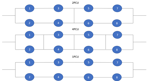
Number of parallel connected units in the module configuration. For example, in a 4s2p battery module 2 parallel connected units means two sub-units of size 2s2p are connected.

electrical_input_type (enumerated) [=current]

Type of global electrical input to battery module.

current: Electric current input. Requires current_type.
c_rate: C-rate input. Requires c_rate_type.
voltage: Voltage input. Requires voltage_type = constant.
power: Power input. Requires power_type.
standard_charge_profile: Pre-defined charging profile.

current_type (enumerated) [=none]

Type of electrical current input.

constant or const: Constant electrical current. Requires current.
piecewise_linear or linear: Piecewise linear curve fit electrical current profile. Requires curve_fit_values and curve_fit_variable.
cubic_spline or spline: Cubic spline curve fit electrical current profile. Requires curve_fit_values and curve_fit_variable.

current (real) [=0]

Constant value of electrical current. When current_type is constant. Notice you have positive current for discharging and negative current for charging.

current_curve_fit_values (array) [={0,0}]

A two-column array of independent-variable/isotropic electrical current data values. The independent variable is either state of charge or time. Used with piecewise_linear and cubic_spline types.

current_curve_fit_variable (enumerated) [=time]

Independent variable of the curve fit for isotropic electrical current. Used with piecewise_linear and cubic_spline types.

time: time

c_rate_type (enumerated) [=none]

Type of c-rate input.

none: No c-rate type specified.
constant or const: Constant c-rate value. Requires c_rate.
piecewise_linear or linear: Piecewise linear curve fit c-rate profile. Requires curve_fit_values and curve_fit_variable.
cubic_spline or spline: Cubic spline curve fit c-rate profile. Requires curve_fit_values and curve_fit_variable.

c_rate (real) [=0]

Constant value of c-rate. When type is constant.

c_rate_curve_fit_values (array) [={0,0}]

A two-column array of independent-variable/isotropic c-rate data values. The independent variable is time. Used with piecewise_linear and cubic_spline types.

c_rate_curve_fit_variable (enumerated) [=time]

Independent variable of the curve fit for isotropic c-rate. Used with piecewise_linear and cubic_spline types.

time: time

voltage_type (enumerated) [=constant]

Type of voltage input.

constant or const: Constant voltage value. Requires voltage.

voltage (real) [=0]

Constant value of module input voltage. When voltage_type = constant.

power_type (enumerated) [=constant]

Type of power input.

constant or const: Constant power value. Requires power.
piecewise_linear or linear: Piecewise linear curve fit power profile. Requires curve_fit_values and curve_fit_variable.
cubic_spline or spline: Cubic spline curve fit power profile. Requires curve_fit_values and curve_fit_variable.

power (real) [=0]

Constant value of module input power. When power_type = constant. Input can be positive or negative.

power_curve_fit_values (array) [={0,0}]

A two-column array of independent-variable/isotropic power data values. The independent variable is time. Used with piecewise_linear and cubic_spline types.

power_curve_fit_variable (enumerated) [=time]

Independent variable of the curve fit for power. Used with piecewise_linear and cubic_spline types.

time: time

charging_profile_type (enumerated) [=none]

Type of power input.

none: No charging profile used.
constant_current_constant_voltage or cccv: Constant current constant voltage charging profile. Requires a module input current or c_rate to be specified.
constant_power_constant_voltage or cpcv: Constant power constant voltage standard charging profile. Requires module power to be specified.

cut_off_current_percent (real) [=0.01]

Current at which the battery is considered fully charged when using charge profiles.

maximum_cell_voltage (real) [=4.20]

Maximum allowed voltage of an individual battery cell. This avoids overcharging.

minimum_cell_voltage (real) [=3.0]

Minimum allowed voltage of an individual battery cell.

maximum_cell_state_of_charge (real) [=0.95]

State of charge at which a battery cell is considered fully charged.

minimum_cell_state_of_charge (real) [=0.05]

State of charge at which a battery cell is considered fully discharged.

module_id (int) ≥ 0 [=1]

Module ID of battery module in a pack.

battery_pack (string) [=no default]

User-given name of the BATTERY_PACK to which this BATTERY_MODULE belongs.

Description

Battery Modules and Components

The BATTERY_MODULE command specifies parameters related to a battery module (multiple battery cells connected in series and parallel).

BATTERY_MODULE commands are referenced by BATTERY_COMPONENT_MODEL commands, which in turn are referenced by an ELEMENT_SET command.

BATTERY_MODULE( "4s2p battery module" ) {
        number_of_parallel_cells = 2
        number_of_serial_cells = 4
        electrical_input_type = current
        current_type = constant
        current = 20
        number_of_parallel_connected_units = 2
}
BATTERY_COMPONENT_MODEL( "battery cell" ) {
   battery_module = "4s2p battery module"
   ...
}

BATTERY_COMPONENT_MODEL( "battery positive terminal" ) {
   battery_module = "4s2p battery module"
   ...
}

ELEMENT_SET( "battery cell element set" ) {
   Battery_component_model = "battery cell"
   ...
}
ELEMENT_SET( "terminal element set" ) {
   Battery_component_model = "battery positive terminal"
   ...
}

Cell Electrical Connectivity

The number of parallel and serial cells, number_of_parallel_cells and number_of_serial_cells respectively, are defined by their electrical connectivity, for example a pouch module made up of 8 cells in a 4s2p configuration would be:

Where four pairs of parallel connected cells: 1&2, 3&4, 5&6, and 7&8, are connected in series to make up the module configuration 4s2p. Alternatively, for a cylindrical module, with 48 cells in an 8s6p configuration:

Each set of 6 cells, for example, 1-6 or 7-12, are connected in parallel. These banks of parallel cells are then connected in series, for example, cells 1-6 are connected in series to cells 7-12. The number_of_parallel_connected_units is how many PCUs (parallel connected unit) you have in the configuration. Conceptually a PCU and an SCU, given by PCU being equal to the number of serial connected cells, is demonstrated in the following figure:

For example, in a 4s2p case, where the number_of_parallel_connected_units = 1, 2 or 4. The corresponding electrical connection of the battery cells would be:

Multi-Battery Module Treatment

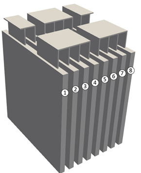
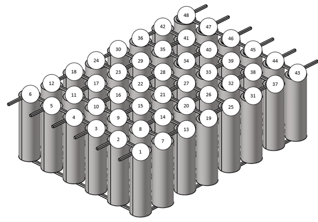
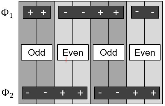
In a battery module, batteries are connected in a nSmP pattern, for example, 8s6p, where m batteries are connected in parallel and then n of these parallel connected units are connected in serial to form a pack. In the MSMD method, two potential equations are solved for the

ϕ_{1}

and

ϕ_{2}

electrical field. Depending on battery connectivity,

ϕ_{1}

and

ϕ_{2}

could be the potential from the positive current collector or the negative one. Therefore, in a battery module simulation, the two potential equations are solved with the transfer current density changing sign dependent on the location in the module. The cells are alternating as odd and even stages. See figure 4. In tabs and busbars, you only solve for one of the fields. In figure 4, the

ϕ_{1}

and

ϕ_{2}

on the left indicates which field was solved in the tabs/busbars in the line. The governing equations for the cell scale become:(1)

\nabla (σ \nabla ϕ) = j

For

ϕ_{1}

in an odd stage:(2)

σ = σ_{+}

(3)

j = - I / V

For

ϕ_{1}

in an even stage:(4)

σ = σ_{-}

(5)

j = I / V

For

ϕ_{2}

in an odd stage:(6)

σ = σ_{-}

(7)

j = I / V

For

ϕ_{2}

in an even stage:(8)

σ = σ_{+}

(9)

j = - I / V

Cell Current/Voltage Calculation in Module

To model serial and parallel connected modules, state and model information is needed for each individual cell. The module current

I^{k}

is given, but the individual current through each battery (

I_{j}^{k}

) is needed for the electric potential equation, energy equation, ECM model, and the voltage across each PCU as the reference potential. As an example, suppose two PCUs are connected in series. Then the electrical circuit diagram would be as follows:

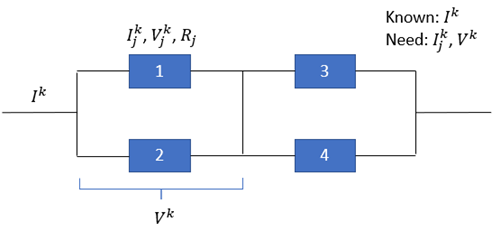
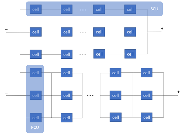
To get current and voltage distribution over each cell, the terminal voltage is separated into a "fixed" part (

V_{j}^{k}

) and a "variable" part.(10)

V = V_{fixed} + V_{variable}

(11)

V_{fixed} = V_{o c} - \sum_{i} R_{i} I_{R}^{k} = V_{j}^{k}

(12)

V_{variable} = R_{0} I_{j}^{k}

Everything is known for the "fixed" part from the last time step, the reference potential V^k can be calculated across any PCU based on the following equation. I^k is the pack charging/discharging current, which is an input.(13)

V^{K} = \frac{\sum_{j} \frac{V_{j}^{k}}{R_{j}} - I^{k}}{\sum_{j} \frac{1}{R_{j}}}

(14)

I_{j}^{k} = \frac{V_{j}^{k} - V_{k}}{\sum_{j} R_{s, j}}

I_{j}^{k} I_{R}^{k} I_{j}^{k}

is then used in the subscale model to calculate

I_{R}^{k}

R_{1}

C_{1}

is the polarization resistance and capacitance from the first pair,

R_{2}

C_{2}

is the polarization resistance and capacitance from the second pair,

I_{R_{1}}^{k}

I_{R_{2}}^{k}

I_{R_{1}}^{k + 1}

I_{R_{2}}^{k + 1}

are diffusion resistor current at time step k and k+1.(15)

I_{R_{1}}^{k + 1} = \exp (\frac{- Δ t}{R_{1} C_{1}}) I_{R_{1}}^{k} + (1 - \exp (\frac{- Δ t}{R_{1} C_{1}})) I_{j}^{k}

(16)

I_{R_{2}}^{k + 1} = \exp (\frac{- Δ t}{R_{2} C_{2}}) I_{R_{2}}^{k} + (1 - \exp (\frac{- Δ t}{R_{2} C_{2}})) I_{j}^{k}

Electrical Input Type

Different types of electrical input can be included as an input to the battery module using the electrical_input_type command. These are summarized in the following sections.

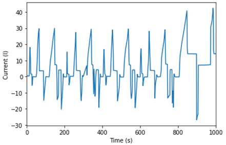
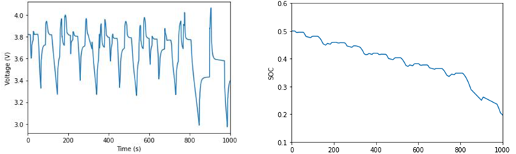
Current

Current supports both generic charging and discharging, these include: constant; piecewise_linear; cubic_spline; and current profiles.

The following gives an example input for a current profile:

BATTERY_MODULE( "4S2P battery module" ) {
    number_of_parallel_cells = 2
    number_of_serial_cells = 4
    electrical_input_type = current
    current_type = piecewise_linear
    current_curve_fit_values = Read( "time_current.txt" )
    current_curve_fit_variable = time
    cut_off_current_percent = 0.1
    maximum_cell_voltage = 4.2
    minimum_cell_voltage = 2.7
    minimum_cell_state_of_charge = 0.05
    maximum_cell_state_of_charge = 0.95
}

And time_current.txt would look like this:

0               0.66809696
9.61104062      0.66809696       
12.5842409      0.66809696
13.34691228     15.37136268
…

Figure 7 shows a typical driving profile with current input. Figure 8 shows the voltage and soc response from this particular current input. The driving profile is taken from [1].

[1] Mahfoudi, Nadjiba, et al. "Thermal Analysis of LMO/Graphite Batteries Using Equivalent Circuit Models." Batteries 7.3 (2021): 58.

C-Rate

C-rate supports both generic charging and discharging, these include: constant; piecewise_linear; cubic_spline; and c-rate profiles.

C-rate is the speed at which a battery is charged/discharged. For example, if you have a battery with a capacity of 3.5Ah, then you can calculate how many amps it can provide for different charging or discharging rates. Below are some examples:

Battery with capacity of 3.5Ah discharged at a c rate of 0.5C delivers 1.75A for 2 hours.
Battery with capacity of 3.5Ah discharged at a c rate of 1C delivers 3.5A for 1 hour.
Battery with capacity of 3.5Ah discharged at a c rate of 2C delivers 7A for 30 mins.

To define a constant c-rate for a 1C discharge the BATTERY_MODULE would be:

BATTERY_MODULE( "4s2p battery module" ) {
    number_of_parallel_cells = 2
    number_of_serial_cells = 4    
    electrical_input_type = c_rate
    c_rate = 1
    number_of_parallel_connected_units = 2
}

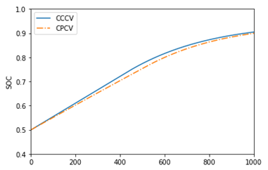
Charging Profiles

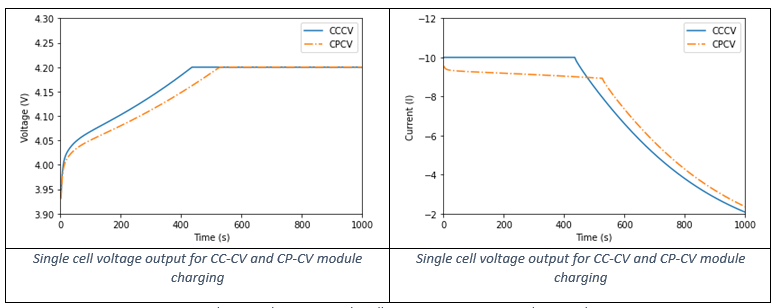
For charging profiles, you can have CC-CV or CP-CV. For CC-CV the charging starts with a constant current, or c_rate, and then switches to a constant voltage charging method once the voltage limit is reached. The simulation will terminate when the current drops to a pre-defined level, for example, minimum current or maximum soc. For CP-CV, the initial charging is constant power and switches to constant voltage once the voltage limit is reached. The CP-CV charging terminates in the same manner as CC-CV. A typical CC-CV or CP-CV charging current, voltage and soc curve are shown in the following figures.

Example CC-CV input: For a CC-CV input, the following parameters need to be defined:

electrical_input_type = standard_charge_profile
charging_profile_type = constant_current_constant_voltage
current/c_rate

The following parameters can typically be taken to be default:

cut_off_current_percent
maximum_cell_voltage
minimum_cell_voltage
minimum_cell_state_of_charge
maximum_cell_state_of_charge

BATTERY_MODULE( "4S2P battery module" ) {
    number_of_parallel_cells = 2
    number_of_serial_cells = 4
    electrical_input_type = standard_charge_profile
    charging_profile_type = constant_current_constant_voltage
    current_type = constant    
    current = -20
    cut_off_current_percent = 0.1
    maximum_cell_voltage = 4.2
    minimum_cell_voltage = 3.0    
    minimum_cell_state_of_charge = 0.05    
    maximum_cell_state_of_charge = 0.95
}

Example input CP-CV: The input for CP-CV the following parameters need to be defined:

electrical_input_type = standard_charge_profile
charging_profile_type = constant_power_constant_voltage
power

The following parameters can typically be taken to be default:

cut_off_current_percent
maximum_cell_voltage
minimum_cell_voltage
minimum_cell_state_of_charge
maximum_cell_state_of_charge

BATTERY_MODULE( "4S2P battery module" ) {	
    number_of_parallel_cells = 2
    number_of_serial_cells = 4
    electrical_input_type = standard_charge_profile
    charging_profile_type = constant_power_constant_voltage
    power_type = constant
    power = 300
    cut_off_current_percent = 0.1
    maximum_cell_voltage = 4.2
    minimum_cell_voltage = 3.0
    minimum_cell_state_of_charge = 0.05
    maximum_cell_state_of_charge = 0.95
}

Constant Power (CP)

CP is charging with constant power, for example, power_type = constant.

Example input CP: For a CP input, the following parameters need to be defined:

electrical_input_type = power
power

The following parameters can typically be taken to be default:

cut_off_current_percent
maximum_cell_voltage
minimum_cell_voltage
minimum_cell_state_of_charge
maximum_cell_state_of_charge

BATTERY_MODULE( "4S2P battery module" ) {
    number_of_parallel_cells = 2
    number_of_serial_cells = 4
    electrical_input_type = power
    power_type = constant
    power = 300
    cut_off_current_percent = 0.1
    maximum_cell_voltage = 4.2
    minimum_cell_voltage = 2.7
    minimum_cell_state_of_charge = 0.05
    maximum_cell_state_of_charge = 0.95
}

Constant Voltage (CV)

CV is charging with constant voltage, for example, voltage_type = constant. The input module voltage divided by the number of parallel cells should be between the minimum and maximum cell voltage.

Example input CV: For a CV input, the following parameters need to be defined:

electrical_input_type = voltage
voltage

BATTERY_MODULE( "4S2P battery module" ) {
    number_of_parallel_cells = 2
    number_of_serial_cells = 4
    electrical_input_type = voltage
    voltage_type = constant
    voltage = 16
    cut_off_current_percent = 0.1
    maximum_cell_voltage = 4.2
    minimum_cell_voltage = 2.7
    minimum_cell_state_of_charge = 0.05
    maximum_cell_state_of_charge = 0.95
}