
hilbert
Hilbert transform.
Syntax
h = hilbert(x)
h = hilbert(x,n)
h = hilbert(x,n,dim)
Inputs
- x
- The real signal to be transformed into an analytic signal.
- n
- Size of the transform.
- dim
- The dimension on which to operate.
Outputs
- h
- The analytic extension for x.
Example
Perform envelope detection of a real signal using the Hilbert transform.
fs = 4000; % sampling frequency
ts = 1/fs; % sampling time interval
n = 800; % number of samples
t = [0:ts:(n-1)*ts]; % time vector
signal = sin(2*pi*25*t) + 0.8 * sin(2*pi*40*t);
carrier = cos(2*pi*200*t);
sigmod = signal .* carrier;
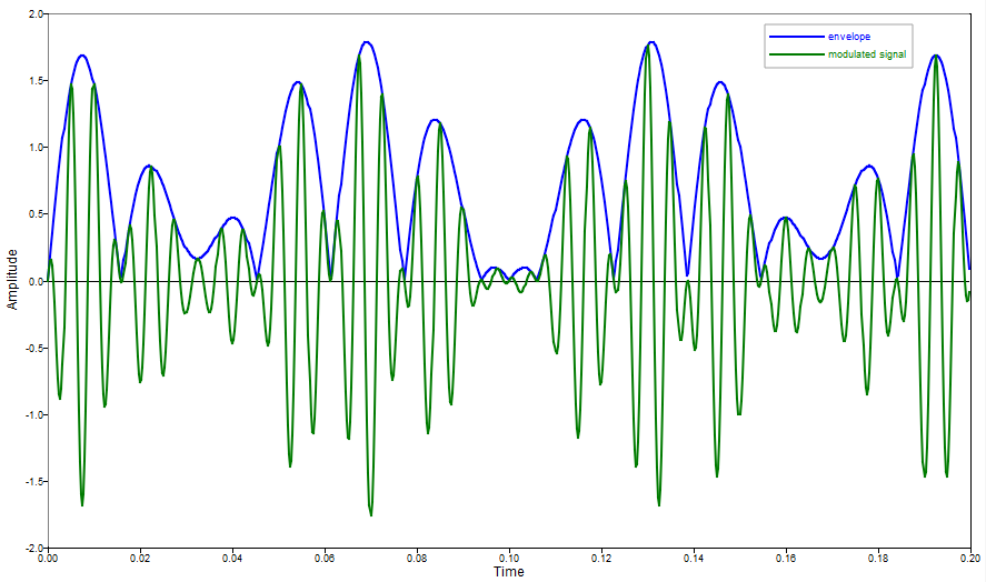
h = hilbert(sigmod);
plot(t, signal, 'b');
hold on;
plot(t, sigmod, 'color', [0,123,0]);
xlabel ('Time');
ylabel ('Amplitude');
legend('signal','modulated signal');
figure;
plot(t, abs(h), 'b');
hold on;
plot(t, sigmod,'color',[0,123,0]);
xlabel ('Time');
ylabel ('Amplitude');
legend('envelope','modulated signal');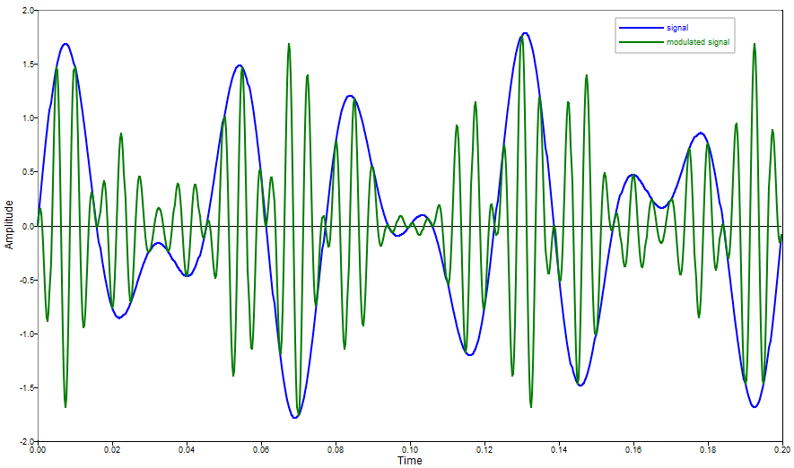
Comments
The analytic representation is useful in facilitating certain other processing operations. The real component of the transform matches the input signal. The imaginary component contains its Hilbert transform.
Envelope detection takes advantage of a 90 degree phase shift that occurs with the Hilbert transform. The shift causes the carrier frequency to drop out when taking the magnitude, leaving only the signal envelope.