The numerator polynomial coefficients of the filter.
Type: double
Dimension: vector
a
The denominator polynomial coefficients of the filter.
Type: double
Dimension: vector
n
The number of frequencies at which to compute the delay.
For frequencies in Hz, when 'whole' is specified the range is
[0,fs), and [0,fs/2) otherwise. For normalized angular frequecies
in radians, when 'whole' is specified the range is [0, 2*pi),
and [0,pi) otherwise.
Default: 512 (use []).
Type: integer
Dimension: scalar
f
The frequencies (in Hz) at which the delay is computed.
Type: double
Dimension: scalar | vector
w
The normalized angular frequencies (in radians) at which the delay is
computed. The normalized Nyquist frequency is pi radians.
Type: double
Dimension: scalar | vector
fs
The sampling frequency (in Hz).
Type: double
Dimension: scalar
Outputs
gd
The group delay values in units of samples.
Type: double
Dimension: scalar | vector
f
The frequencies (in Hz) at which the delay is computed.
Type: double
Dimension: scalar | vector
w
The normalized angular frequencies (in radians) at which the delay is computed.
Type: double
Dimension: scalar | vector
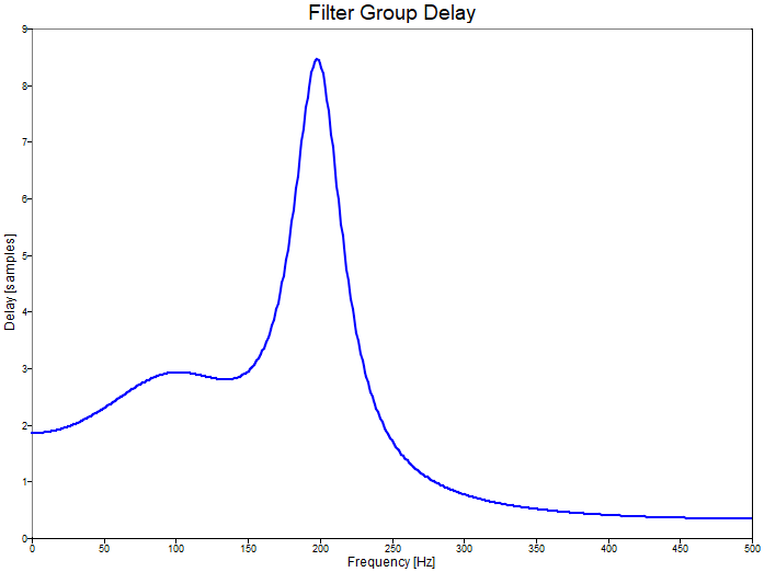
Example
Plot the group delay of a fourth order Chebyshev I low pass digital filter with a
200 Hz cutoff frequency and a 1000 Hz sampling frequency.
fc = 200;
fs = 1000;
[b,a] = cheby1(4,1,fc/(fs/2));
grpdelay(b,a,[],fs);
Figure 1. fft figure 1
Comments
With no return arguments, the function will automatically plot.
A warning is issued if the time delay does not exist for some computed frequency value,
in which case the delay is reported as zero. A common scenario for this is when the delay
is computed at the Nyquist frequency.