
rlocfind
Find gain and poles for specific points of a root locus diagram.
Syntax
rlocfind(sys)
[k, poles] = rlocfind(sys)
[k, poles] = rlocfind(sys, pe)
Inputs
- sys
- A linear time-invariant transfer function or state space system.
- pe
- A pole estimate from which to compute actual poles with the same gain magnitude.
Outputs
- k
- The gain magnitude associated with pe.
- poles
- The poles on the root locus with gain k.
Examples
s = tf('s');
GH = (s^2 + 2*s + 2) / (s * (s^4 + 9*s^3 + 33*s^2 + 51*s + 26));
[k, poles] = rlocfind(GH, -1+3i)
k = 45.1559797
p = [Matrix] 5 x 1
-5.60380 + 0.00000i
-0.91234 + 2.92420i
-0.91234 - 2.92420i
-0.78576 + 1.04887i
-0.78576 - 1.04887iUse the interactive mode to find the poles for the selected point:
s = tf('s');
GH = (s^2 + 2*s + 2) / (s * (s^4 + 9*s^3 + 33*s^2 + 51*s + 26));
[k, poles] = rlocfind(GH)
Click on the plot to select a point. In this example, point -1+3i is selected and the calculated gain and poles are printed in the console:
Selected point =
-1.00136995 + 3.00236011i
K = 45.1862
poles =
[Matrix] 5 x 1
-5.60471 + 0.00000i
-0.91172 + 2.92491i
-0.91172 - 2.92491i
-0.78593 + 1.04889i
-0.78593 - 1.04889i
The closed loop poles are plotted and the gain, damping and frequency values are displayed in a text box.
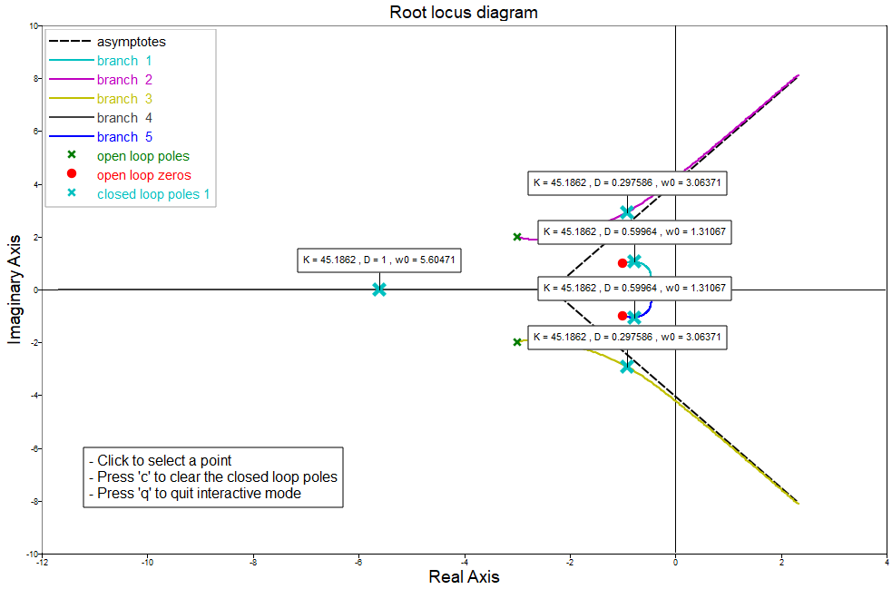
You may click again on the plot to select another point, press 'c' to remove the closed loop poles from the plot or press 'q' to quit the interactive mode. The outputs of interactive rlocfind are the gain and poles of the last selected point
Comments
If pe is omitted, the function enters the interactive mode, which allows the user to select a pole estimate from an existing root locus plot using the mouse.