Tutorial: Immersion Quenching Analysis
Tutorial Level: Beginner Set up and run an immersion quenching analysis, then interpret the results.
Quenching, in the context of the metal extrusion process, is a rapid cooling process used to reduce the temperature of the extruded profile to handling temperature levels. Typically, the extruded aluminum profile exits the die in the range of 500 – 575° C; the goal is to reduce this to approximately 50° C (suitable for handling). In addition, the quenching process is designed to achieve desirable microstructure.
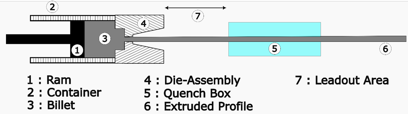
The extruded profile is passed through a series of quench systems. For aluminum extrusion, immersion, water spray, air nozzle, and air fan quench systems are used. These systems can be used in combination and Inspire Extrude can model such combinations.
The temperature and the grain size distribution at the exit of the die form an important process input for the analysis. It is possible to extract this data from a prior extrusion analysis (not illustrated in this tutorial). The area between the exit of the die and the first quench system is denoted as the leadout length and used as a process parameter. In addition, each type of quench system requires a specific set of data corresponding to it.
Objectives: Set up and run an immersion quenching analysis and interpret the results.
Open the Tutorial Model
- From the menu bar, select .
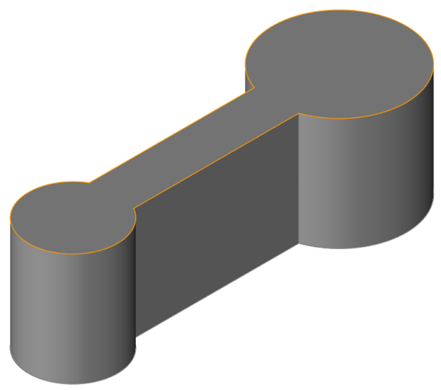
- Browse to your working directory, select dumbbell_profile.x_t, and click Open.
-
Position the model as shown.
- Set the display units to Metric (mm kg MPa C s).
Orient the Model
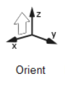
Inspire Extrude assumes the extruded profile comes in a positive Z axis. These steps help to orient the profile in this axis automatically.
- On the ribbon, click the Quenching tab.
-
Click the Orient icon.
-
On the model, click the exit surface.
The model is oriented such that the profile is in the +Z direction.
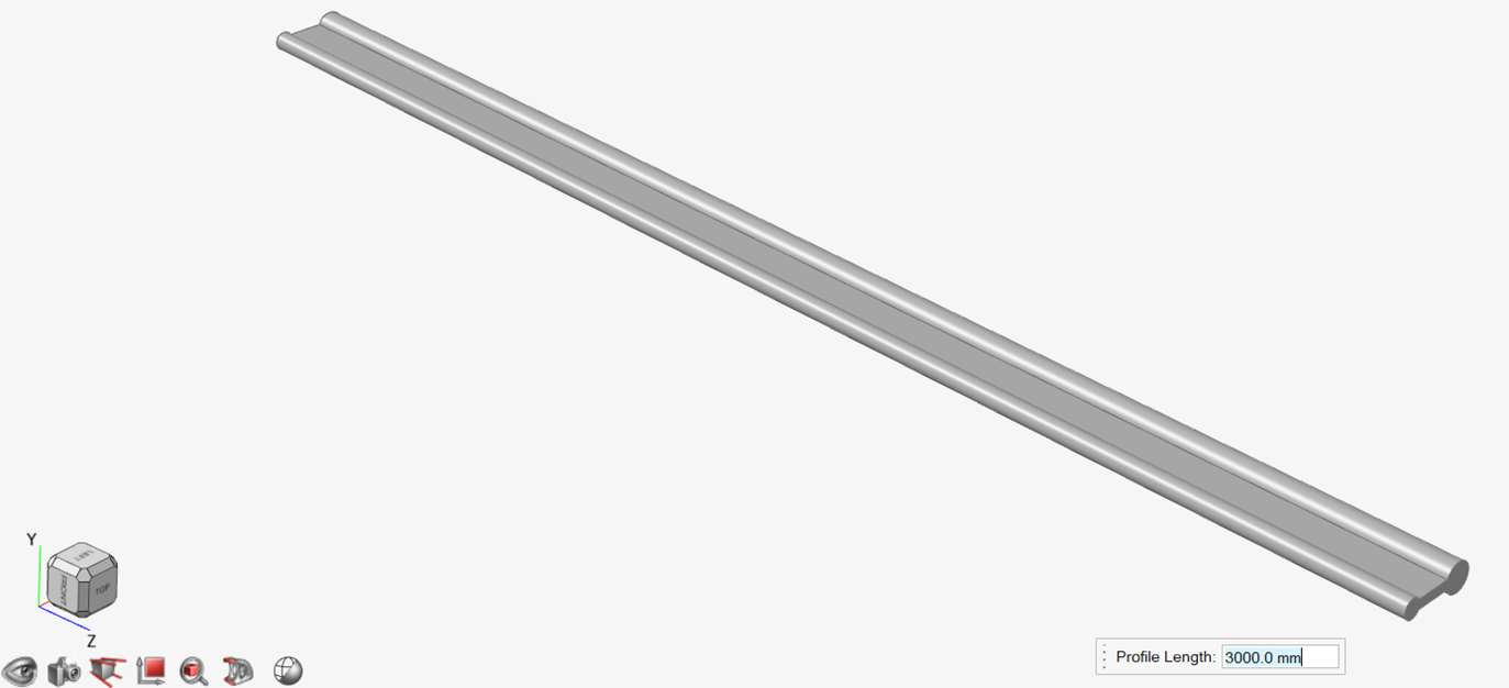
Create the Extruded Profile
The imported or created profile cross-section often does not have the desired length of the extruded profile, which is achieved in this step.
-
From the Quenching ribbon, click the
Profile icon.

-
On the model, click the exit surface as shown.
- Enter 3000 mm for Profile Length.
Create an Immersion Quenching Zone
-
On the Quench icon, click the Create Quench
System satellite.

-
Click the Immersion icon.

-
Change the quench box length L to 1000
mm.
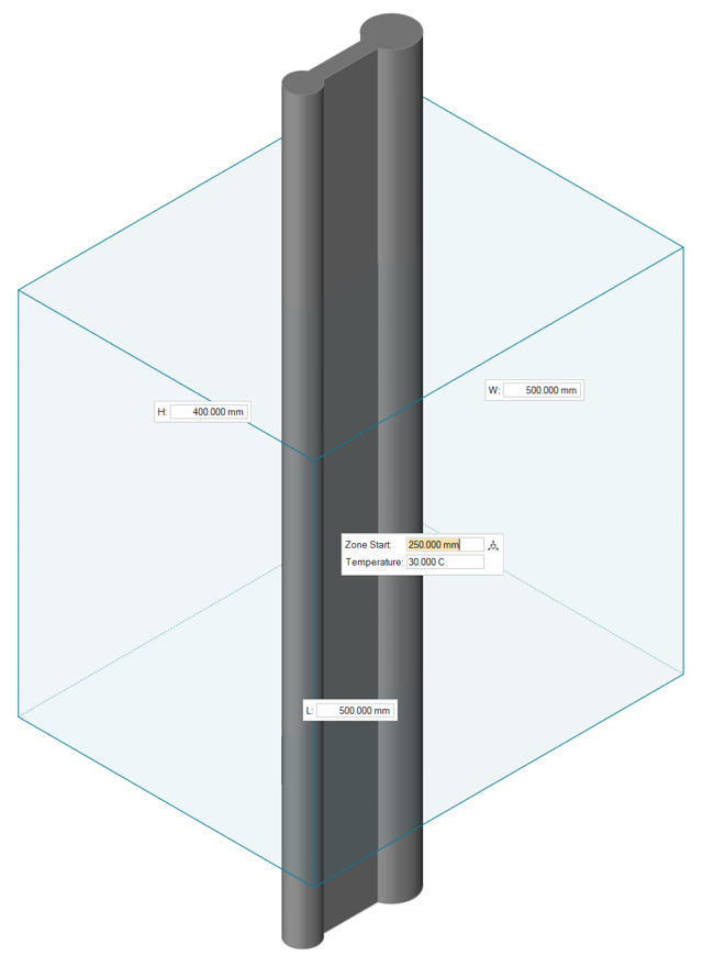
Note: Ensure the zone start is not 0 mm. This value provides the essential distance between the die opening and the quench box, where the leadout table is positioned.
Review Material Properties
-
Click the Materials icon.

-
Ensure that you are using the default material data for this analysis.
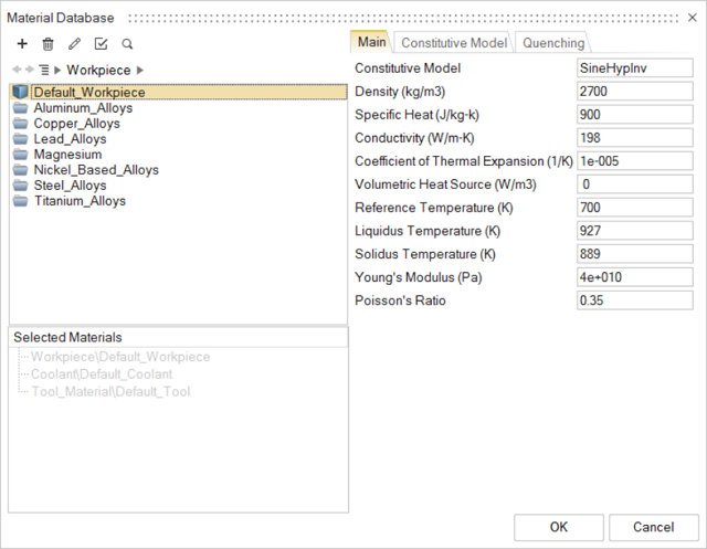
- Click OK to confirm.
Run a Quenching Analysis
- Save the model.
-
Click the Run Analysis icon.

-
Enter and review the following parameters for the Quenching Analysis:
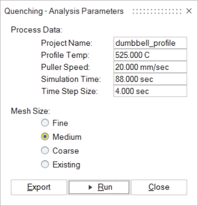
- Click Run.
Review the Quenching Results
- When the analysis is complete, double-click the name of the run to open the results.
- In the Analysis Explorer, select the Temperature result type.
-
Click the Play button in the animation ribbon.
Figure 2. Temperature Distribution over Profile as it Passes through the Quench Box 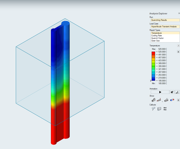
- Select and animate the other result types.
- Right-click to exit the Analysis Explorer.
Figure 2 shows the temporal evolution of temperature as the profile passes through the quench box.
To see the temporal evolution of temperature at any point in the Analysis Explorer, select the Callouts icon. Then select a point where you want to see the temporal evolution. You can choose multiple points as well.
In the Callouts section, click Plots. The temporal evolution of temperature at selected two points is shown.
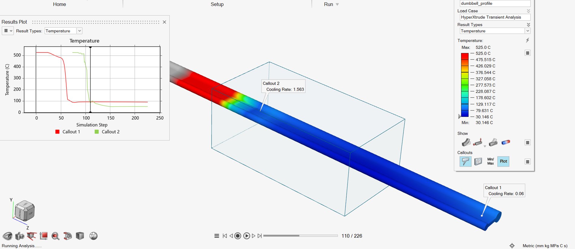
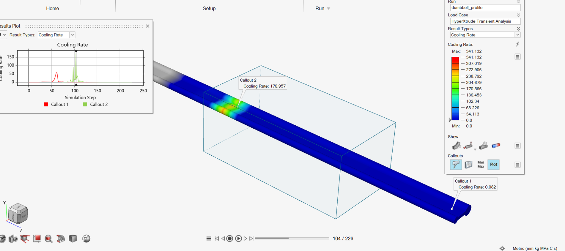
Figure 4 illustrates the temperature evolution at selected points during the cooling process. The cooling occurs in three phases:
- The first phase begins when the hot extruded profile, at approximately 525° C, comes into contact with cold water at 30° C. Upon contact, vapor bubbles form, creating a thin insulating layer around the profile. This vapor layer resists heat transfer, resulting in a slower temperature drop.
- After the profile's temperature sufficiently decreases, the second phase begins. The vapor layer formed in the initial phase breaks down, leading to rapid cooling. This rapid cooling continues until the profile reaches the boiling point of water.
- When the profile's temperature drops below the boiling point of water, the third phase of heat transfer begins, characterized by natural convection. Cooling in this phase is generally slower. By the end of this phase, the extruded profile reaches a handling temperature of 50–70° C.
Faster cooling during quenching can lead to high residual stresses, distortion, or cracking. On the other hand, slower cooling results in an undesirable microstructure with lower strength and hardness in the alloy. The cooling rate during quenching must be optimal to achieve the desired mechanical properties and corrosion resistance.
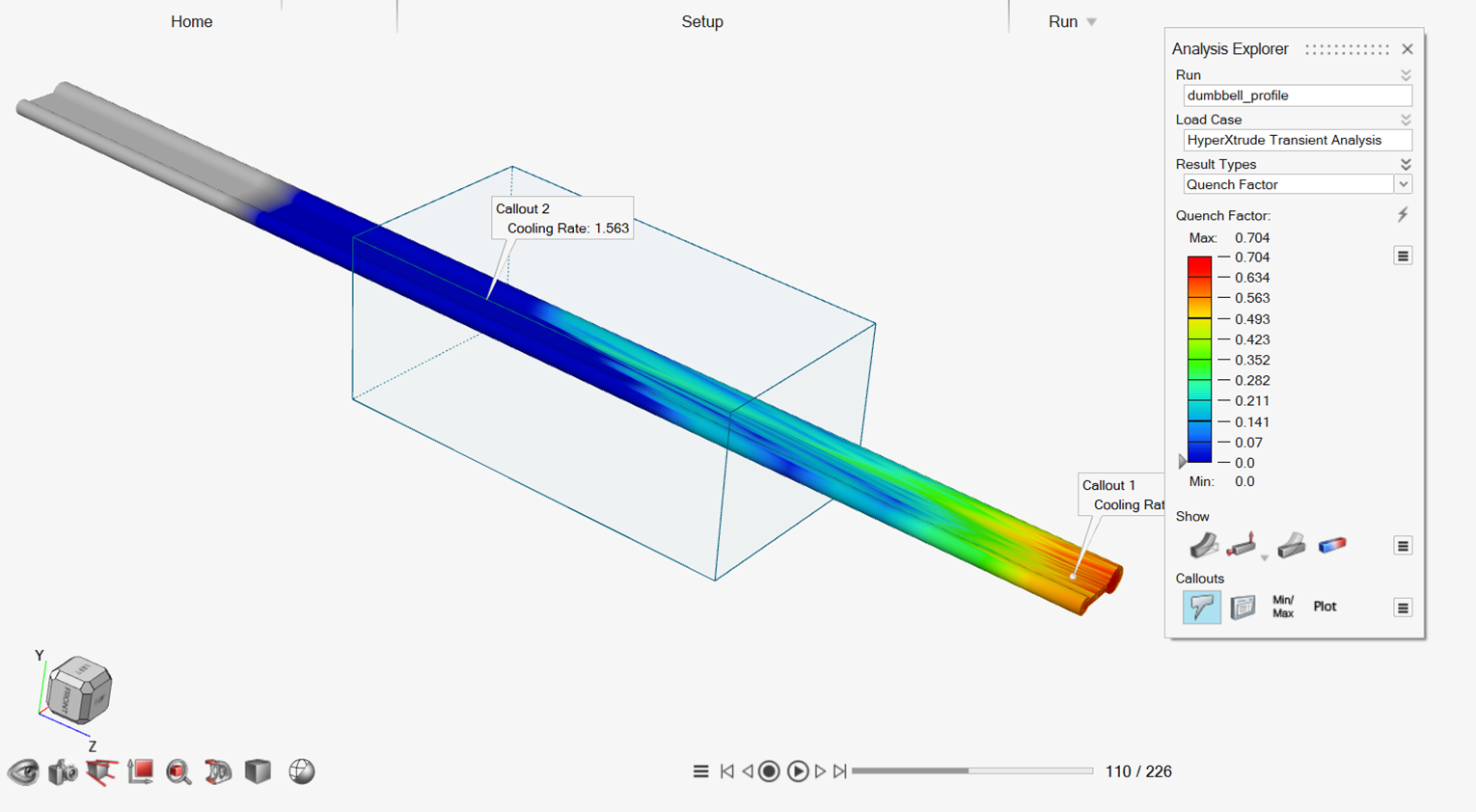
The cumulative Quench Factor (QF) is a non-dimensional quantity that indicates how close the actual cooling rate is to the ideal rate using the critical time determined from the Time-Temperature-Precipitation diagram. The result plotted is cumulative (integral) of the incremental QF computed at each timestep. Low values of QF are associated with high quench rates (cooling happens faster than the critical time) and lead to minimum precipitation and higher yield strengths. On the other hand, higher values lead to lower yield strength. Another important metric is the nonuniformity of QF in the domain.
To analyze QF results, select .