OS-V: 0292 Hertzian Contact - Rigid Sphere and Elastic Half Space, 2D Axisymmetric, S2S Contact
Hertzian contact is demonstrated using OptiStruct for rigid sphere and elastic half-space –2D axisymmetric, S2S CONTACT.
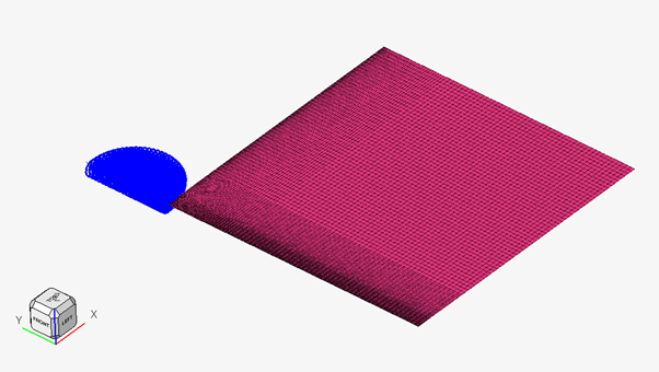
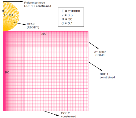
Since the 2D axisymmetric analysis is computationally less expensive compared to 3D analysis, a bigger half space size is used for the 2D axisymmetric analysis. In the model, CQAXI and CTAXI are the elements. Use PAXI and PCONT as card image for the property. See FIGURE for model details.
Model Files
Benchmark Model
Since the 2D axisymmetric analysis is computationally less expensive compared to 3D analysis, a bigger half space size is used for the 2D axisymmetric analysis. In the model, CQAXI and CTAXI are the elements. Use PAXI and PCONT as card image for the property. See Figure 2.
- Material Properties
- Value
- Young's modulus (E)
- 210000
- Poisson's ratio ( )
- 0.3
- R
- 30
- d
- 0.1
Analytical Results:
The analytical solutions are provided by Popov, 2010. The derivation of the analytical solution is beyond the technical scope of this document. Some key variables of the analytical solution are as follows:
- Radius of the sphere.
- Depth of indentation.
- Young's modulus.
- Poisson's ratio.
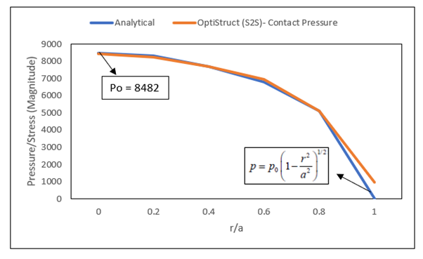
The maximum contact pressure/stress is calculated as:
Results
| Pressure/Stress (Magnitude) | r/a | |
|---|---|---|
| Analytical Result | OptiStruct (S2S)-Contact Pressure | |
| 8482 | 8434 | 0 |
| 8350 | 8272 | 0.2 |
| 7700 | 7696 | 0.4 |
| 6800 | 6960 | 0.6 |
| 5100 | 5110 | 0.8 |
| 0 | 943 | 1 |