Phase 1: Reference Design Synthesis (Free-size Optimization)
In this phase the optimization setup is defined in the concept design phase to identify the stiffest design for the given fraction of the material.
In free-size optimization, the thickness of each designable element is defined as a design variable. Applying this concept to the design of composites implies that the design variables are the thickness of each 'Super-ply' (total designable thickness of a ply orientation) per element.
To obtain more meaningful results, manufacturing constraints are incorporated and
carried through all design phases automatically.
- Objective
- Minimize the compliance of the load case.
- Constraints
- Volume fraction < 0.3
- Design Variables
- Element thicknesses of each ply orientation.
- Manufacturing Constraints
- Ply percentage for the 0s no more than 80% exist.
Set Up the Optimization
Create Free-size Optimization Design Variables
- From the Analysis page, click the optimization panel.
- Click the free size panel.
-
Create the design variable for the free-size optimization.
- Select the create subpanel.
- In the desvar= field, enter free-size.
- Set type to STACK.
- Using the laminates selector, select laminate.
- Click create.
Figure 1. Field Entries for the free-size Panel 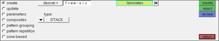
- Select the composites subpanel.
- Click the desvar= field and select free-size.
-
Click edit.
The DSIZE panel opens. In this panel you will define the manufacturing constraints on ply percentage, ply balance, and ply drop-off.
-
Define PLYPCT.
These values constrain the zero- and ninety-degree plies to between twenty and seventy percent of the total thickness of the laminate for any element in the design space.
Figure 2. DSIZE Data Entry Fields for the PLYPCT Cards 
-
Define BALANCE.
Figure 3. DSIZE Data Entry Fields for the BALANCE Card 
-
Define PLYDRP.
Figure 4. DSIZE Data Entry Fields for the PLYDRP Card Using the PLYSLP Method 
- Click return to go back to the composites subpanel.
- Click update.
- Click return and go back to the Optimization panel.
Create Optimization Responses
- From the Analysis page, click optimization.
- Click Responses.
-
Create the volume fraction response.
- In the responses= field, enter Volfrac.
- Below response type, select volumefrac.
- Set regional selection to total and no regionid.
- Click create.
-
Create the compliance response.
- In the response= field, enter compliance.
- Below response type, select compliance.
- Set regional selection to total and no regionid.
- Click create.
- Click return to go back to the Optimization panel.
Create Design Constraints
- Click the dconstraints panel.
- In the constraint= field, enter volfrac.
- Click response = and select volfrac.
- Check the box next to upper bound, then enter 0.3.
- Click create.
- Click return to go back to the Optimization panel.
Define the Objective Function
- Click the objective panel.
- Verify that min is selected.
- Click response= and select compliance.
- Using the loadsteps selector, select nx_step.
- Click create.
- Click return twice to exit the Optimization panel.
Create Output Requests
- From the Analysis page, select the control cards panel.
- In the Card Image dialog, click OUTPUT.
- In the number_of_outputs, enter 3.
-
On the third line, set KEYWORD to FSTOSZ and set FREQ to
YES.
With this keyword, OptiStruct automatically generates a sizing model after free-size optimization.
Figure 5. Requesting the free-size to size (FSTOSZ) optimization output file for Phase 2 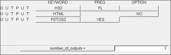
- Click return twice to go back to the Analysis page.
Save the Database
- From the menu bar, click .
- In the Save As dialog, enter oht_opti_ph1.hm for the file name and save it to your working directory.
Run the Optimization
- From the Analysis page, click OptiStruct.
- Click save as.
-
In the Save As dialog, specify location to write the
OptiStruct model file and enter
oht_opti_ph1 for filename.
For OptiStruct input decks, .fem is the recommended extension.
-
Click Save.
The input file field displays the filename and location specified in the Save As dialog.
- Set the export options toggle to all.
- Set the run options toggle to optimization.
- Set the memory options toggle to memory default.
-
Click OptiStruct to run the optimization.
The following message appears in the window at the completion of the job:
OPTIMIZATION HAS CONVERGED.
FEASIBLE DESIGN (ALL CONSTRAINTS SATISFIED).
OptiStruct also reports error messages if any exist. The file oht_opti_ph1.out can be opened in a text editor to find details regarding any errors. This file is written to the same directory as the .fem file. - Click Close.
The default files that get written to your run directory include:
- oht_opti_ph1.out
- OptiStruct output file containing specific information on the file setup, the setup of the optimization problem, estimates for the amount of RAM and disk space required for the run, information for all optimization iterations, and compute time information. Review this file for warnings and errors that are flagged from processing the oht_opti_ph1.fem file.
- oht_opti_ph1_des.h3d
- HyperView binary results file that contain optimization results.
- oht_opti_ph1_s#.h3d
- HyperView binary results file that contains from linear static analysis, and so on.
- oht_opti_ph1_sizing.*.fem
- A ply-based sizing optimization input file generated during free-sizing phase. This resulting deck contains PCOMPP, STACK, PLY, and SET cards describing the ply-based composite model, as well as DCOMP, DESVAR, and DVPREL cards defining the optimization data. The * sign represents the final iteration number.
- oht_opti_ph1_sizing.*.inc
- An ASCII include file contains the same ply-based modeling and optimization data as in the input deck. The * sign represents the final iteration number.
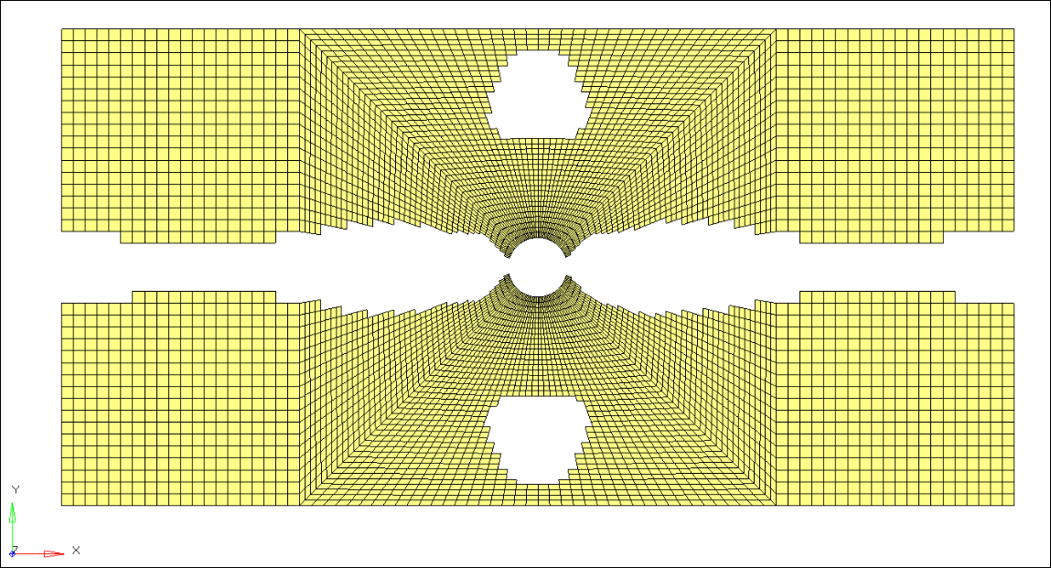
View the Results
View the Element Thickness Results
-
From the OptiStruct panel, click HyperView.
HyperView is launched and the session file oht_opti_ph1.mvw is opened, which contains three pages with the results from two H3D files.
- Page 2
- Optimization results in oht_opti_ph1_des.h3d.
- Page 3
- Analysis results of subcase 1 in oht_opti_ph1_s1.h3d.
Note: If opening these files from standalone HyperMesh, the page numbers will be decremented. - Navigate to the page with the results for oht_opti_ph1_des.h3d.
-
On the Results toolbar, click
 to open the
Contour panel.
to open the
Contour panel.
-
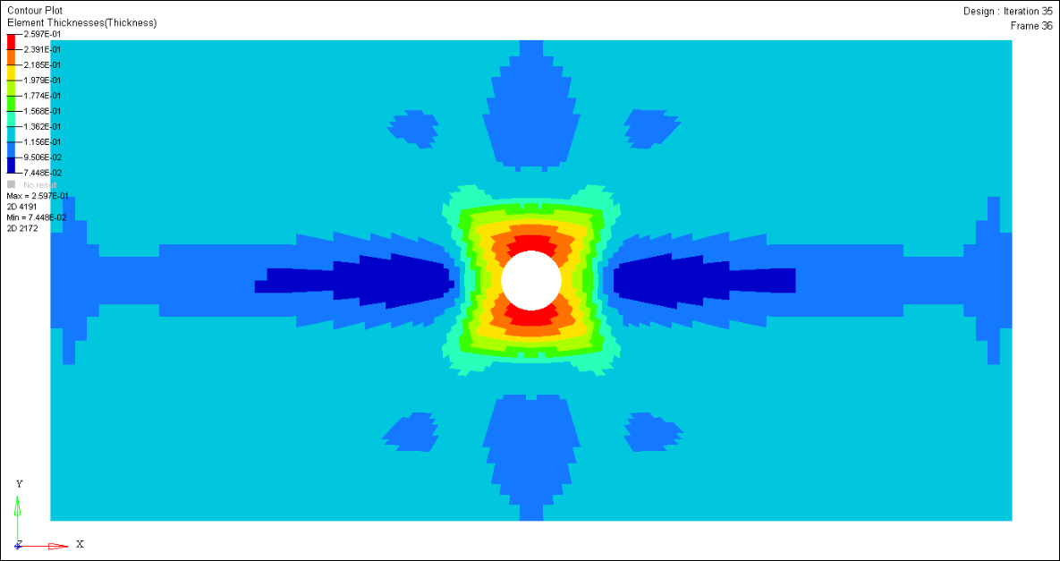
Select the plot options.
Figure 6. Contour panel Plot Options (Free-Size Optimization Results) 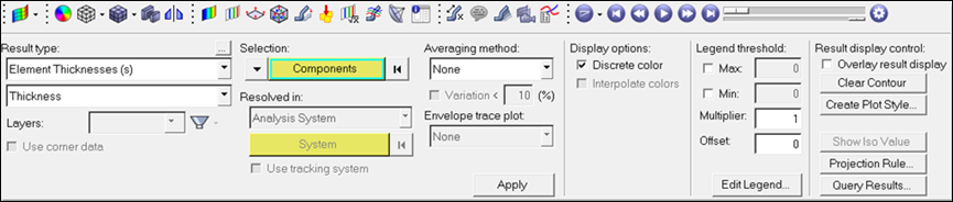
-
In the Results Browser, select the last iteration.
Figure 7. Selecting the Final Iteration 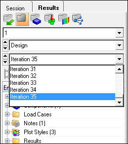
- Click Apply.
-
On the Standard Views toolbar, click
 to view the results in the X-Y plane.
View the Ply Thickness Results
- From the Contour panel, set the Result type to Ply Thicknesses (s).
-
Select the plot options.
Figure 9. Ply Thicknesses Contour Plot 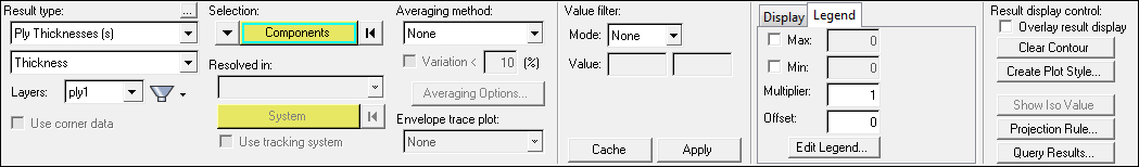
- In the Results Browser, select the last iteration.
-
Click Apply.
The thickness distribution of 0 degree super ply is generated. It represents the ply shapes and patch locations of the 0 degree ply bundles.
Figure 10. Ply Thickness Contour Plot of the 0 Degree Super-Ply 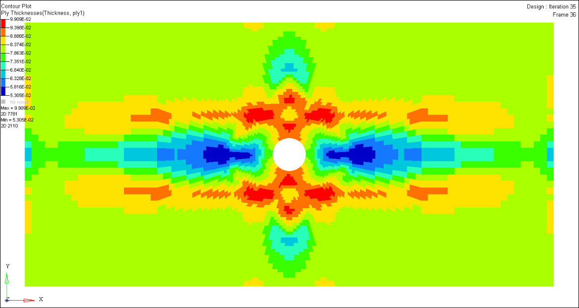
-
Create the ply thickness contours for super-ply 2 (45°), ply 3 (-45°), and ply
4 (90°) by selecting Layers 2, 3 and 4, respectively in the Contour panel.
Due to the balance constraint applied, the thickness distribution of the +45° and the -45° super ply are the same.
Figure 11. Ply Thickness Contour Plot of the -45/+45 Degree Super-ply 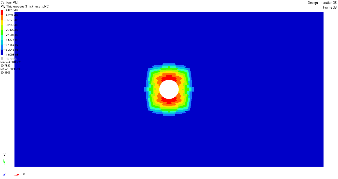
Figure 12. Ply Thickness Contour Plot of the 90 Degree Super-ply 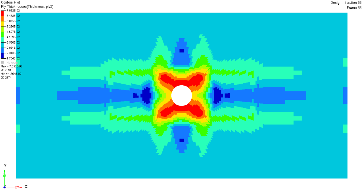
View the Ply Bundles
- Go back to the HyperMesh and start a new model.
- Import the solver deck oht_opti_ph1_sizing.*.inc, located in the same directory where the file oht_opti_ph1.fem, into the current session.
-
In the Model Browser, right-click on the Load
Collectors folder and select Hide from
the context menu.
The display of all load collectors is turned off.
-
In the Model Browser, right-click on the
Plies folder and select Hide
from the context menu.
The display of all plies is turned off.
-
In the Model Browser, Plies folder, activate the mesh view
icon for each ply individually to review the plies.
Figure 13. Model Browser View Showing Ply 11300 Selected (Laminate 1, Ply 1, Shape 3) 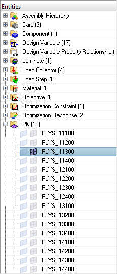
Figure 14. Graphics Area View of Ply 11300 (Laminate 1, Ply 1, Shape 3) 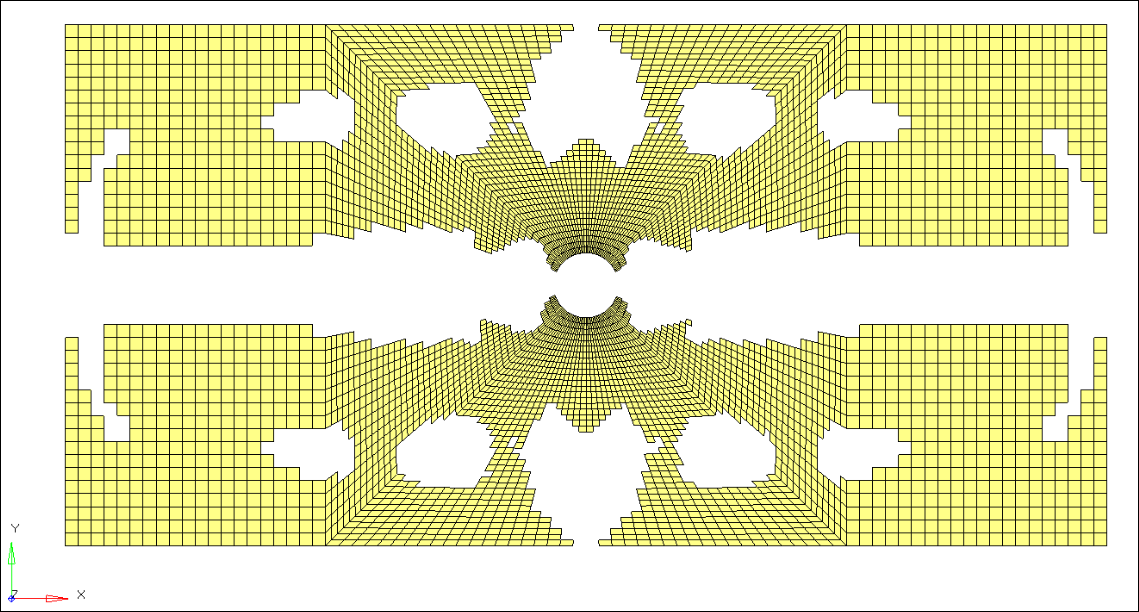
Apply Ply Smoothing using OSSmooth
- From the Post page, click the OSSmooth panel.
- In the Select model field, select oht_opti_ph1_sizing.35.fem.
- Change the mode from Geometry to PLY Shape.
- In the output file field, select the original location with the name of oht_opti_ph1_sizing.35.smoothed.fem.
- In the smooth iterations field, enter 20.
- Under small region, clear the split disconnected and create geometry checkboxes.
- In the area ratio field, enter 0.010.
- Click OSSmooth to run the analysis to smooth the model.