OS-T: 3100 Combined Topology and Topography Optimization of a Slider Suspension
In this tutorial you will perform a combined topology and topography optimization on a slider suspension using OptiStruct.
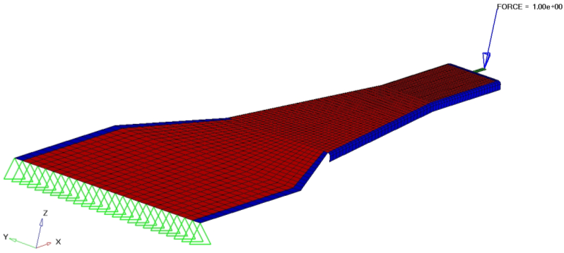
The objective of this tutorial is to increase the stiffness of the slider suspension and make it lighter at the same time. This requires the use of both topology and topography optimization.
- Objective Function
- Minimize the combined weighted compliance and the weighted modes.
- Constraints
- 7th Mode > 12 cycles/ms.
- Design Variables
- Element densities and nodes topography.
Launch HyperMesh and Set the OptiStruct User Profile
-
Launch HyperMesh.
The User Profile dialog opens.
-
Select OptiStruct and click
OK.
This loads the user profile. It includes the appropriate template, macro menu, and import reader, paring down the functionality of HyperMesh to what is relevant for generating models for OptiStruct.
Import the Model
-
Click .
An Import tab is added to your tab menu.
- For the File type, select OptiStruct.
-
Select the Files icon
 .
A Select OptiStruct file browser opens.
.
A Select OptiStruct file browser opens. - Select the combined.fem file you saved to your working directory.
- Click Open.
- Click Import, then click Close to close the Import tab.
Set Up the Optimization
Create Topology Design Variables
- From the Analysis page, click optimization.
- Click topology.
- Select the create subpanel.
- In the desvar= field, enter pin.
- Set type: to PSHELL.
- Using the props selector, select 1pin.
-
Verify that the base thickness is 0.0.
A value of 0.0 implies that the thickness at a specific element can go to zero, and therefore becomes a void.
- Click create.
- Repeat the above steps to create a design variable labeled bend, and assign it the 3bend property.
- Click return.
Define Topography Design Variables
For a topography optimization, a design space and a bead definition need to be defined.
- From the Analysis page, click the optimization panel.
- Click the topography panel.
-
Create a topography design space definition.
- Select the create subpanel.
- In the desvar= field, enter tpg.
- Using the props selector, select 1pin and 3bend.
- Click create.
A topography design space definition, tpg, has been created. All elements organized into the 1pin and 3bend component collector(s) are now included in the design space. -
Create a bead definition for the design space tpg.
A bead definition has been created for the design space tpg. Based on this information, OptiStruct will automatically generate bead variable definitions throughout the design variable domain.
-
Adding pattern grouping constraints.
Use 1-plane symmetric beads, as it is the simplest and can be symmetric at the same time.
- Select the pattern grouping subpanel.
- Click desvar = and select tpg.
- Set the pattern type to 1-pln sym.
- Click anchor node, and enter 41 in the id= field.
- Click first node, and enter 53 in the id= field.
- Click update.
-
Update the bounds of the design variable.
The upper bound sets the upper bound on grid movement equal to UB*HGT and the lower bound sets the lower bound on grid movement equal to LB*HGT.
- Click return to go to the Optimization panel.
Create Optimization Responses
Since this problem is a combined linear static and normal mode analysis, you are trying to minimize compliance and increase frequency for the two load cases, while constraining the seventh frequency. Therefore, two responses are defined: freq and comb.
- From the Analysis page, click optimization.
- Click Responses.
-
Create the frequency response.
- In the responses= field, enter freq.
- Below response type, select frequency.
- For Mode Number, enter 7.0.
- Click create.
A response, freq, is defined for the frequency of the seventh mode extracted. -
Create the compliance index response.
- Click return to go back to the Optimization panel.
Create Design Constraints
- Click the dconstraints panel.
- In the constraint= field, enter frequency.
- Click response = and select freq.
- Check the box next to lower bound, then enter 12.
- Using the loadsteps selector, select frequency.
- Click create.
- Click return to go back to the Optimization panel.
Define the Objective Function
- Click the objective panel.
- Verify that min is selected.
- Click response= and select comb.
- Click create.
- Click return twice to exit the Optimization panel.
Define Optimization Control Cards
- From the Analysis page, click the Optimization panel.
- Click the opti control panel.
-
Select MINDIM, and enter
0.25.
Minimum member size is generally recommended to avoid checkerboarding. It also ensures that the structure has the minimum dimension specified in this card.
-
Select MATINIT, and enter
1.0.
MATINIT declares the initial material fraction in a topology optimization. MATINIT has several defaults based upon the following conditions: If mass is the objective function, the MATINIT default is 0.9. With constrained mass, the default is reset to the constraint value. If mass is not the objective function and is not constrained, the default is 0.6.
- Click return twice to exit the panel.
Set Mode Tracking
- From the Analysis page, click the control cards panel.
- In the Card Image dialog, click PARAM.
- Select MODETRAK.
- Set MODET_V1 to Yes.
-
Click return.
The PARAM button is now green, indicating that it is active.
- Click return to go back to the Analysis page.
Run the Optimization
- From the Analysis page, click OptiStruct.
- Click save as.
-
In the Save As dialog, specify location to write the
OptiStruct model file and enter
comb_complete for filename.
For OptiStruct input decks, .fem is the recommended extension.
-
Click Save.
The input file field displays the filename and location specified in the Save As dialog.
- Set the export options toggle to all.
- Set the run options toggle to optimization.
- Set the memory options toggle to memory default.
-
Click OptiStruct to run the optimization.
The following message appears in the window at the completion of the job:
OPTIMIZATION HAS CONVERGED.
FEASIBLE DESIGN (ALL CONSTRAINTS SATISFIED).
OptiStruct also reports error messages if any exist. The file comb_complete.out can be opened in a text editor to find details regarding any errors. This file is written to the same directory as the .fem file. - Click Close.
View the Results
Post-Process the Shape Results Change (Topography)
-
From the OptiStruct panel, click
HyperView.
HyperView is launched.
-
On the Results toolbar, click
 to open the Deformed panel.
-
Under Deformed shape, define deformed shape settings.
- Set the Result type to Shape Change(v).
- Set Scale to Scale factor.
- Set Type to Uniform.
- In the Value field, enter 1.0.
- Under Undeformed shape, set Show to None.
-
Click Apply.
The shape change due to the topography optimization displays.
-
In the Results Browser, set the Load Case
and Simulation Selection to 25th
iteration.
Figure 2. Topography Result Applied on Slider Suspension 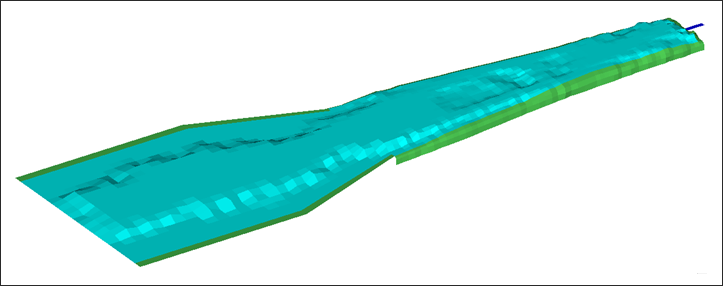
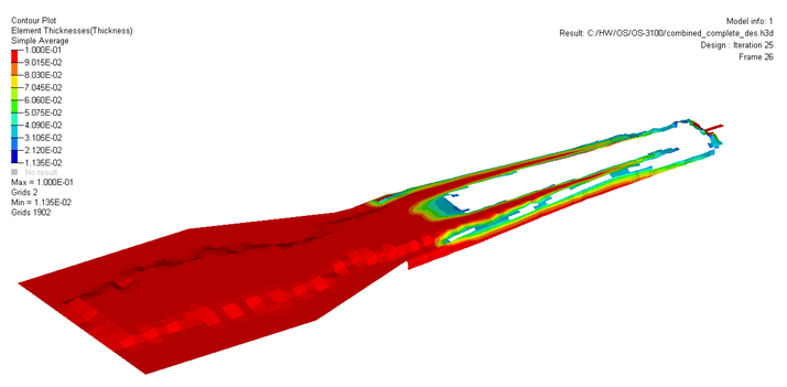
Contour the Optimum Material Distribution (Topologic)
-
On the Results toolbar, click
 to open the Contour panel.
- Set the Result Type to Element Densities (s) and Density.
- Set the Averaging method to Simple.
- Click Apply to display the density contour.
Add Iso Surface of the Optimum Material Distribution (Topologic)
-
On the Results toolbar, click
 to open the Iso Value panel.
- Set the Result Type to Element Densities (s) and Density.
- Set Show values to Above.
- Click Apply to display the density iso-surface plot.
- In the Current value field, enter 0.3.