
ACU-T: 6104 AcuSolve - EDEM Bidirectional Coupling with Non-Spherical Particles
Tutorial Level: Intermediate
This tutorial introduces you to the workflow for setting up and running a basic bidirectional coupling (two-way) simulation with non-spherical particles using AcuSolve and EDEM. Prior to starting this tutorial, you should have already run through the introductory tutorial, ACU-T: 1000 Basic Flow Set Up, and have a basic understanding of HyperMesh CFD, AcuSolve, and EDEM. To run this simulation, you will need access to a licensed version of HyperMesh CFD, AcuSolve, and EDEM.
Problem Description
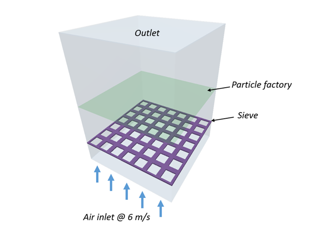
AcuSolve-EDEM bidirectional coupling is used to model the interaction between the fluid and particles. In this tutorial, non-spherical drag force models are used to accurately predict the drag forces on the particles by taking the shape of particles into consideration. The length scale used for factoring in the shape of the particles is the aspect ratio. Bar shaped particles with an aspect ratio of 2.75 and spherical particles with aspect ratio 1 are used for this simulation. The Rong drag model is used in conjunction with the Holzer-Sommerfeld non-spherical drag coefficient model.
| Particle Type | Density (kg/m3) | Size (m) | Number of particles |
|---|---|---|---|
| Bar | 200 | 0.022/0.008 (L/D) | 100 |
| Sphere | 1500 | 0.008 (D) | 200 |
- Isometric – where orientation of the particle is not considered in the drag force calculation. This model is applicable for shapes such as rocks, certain beans and ore particles. The Haider Levenspiel drag model is available for such scenarios and it requires particle’s sphericity and volume as inputs.
- Non-spherical – the orientation of the particle is considered for the drag force calculation. This option is applicable for shapes such as disc, plate and cylinder where the orientation of the particle with respect to the flow velocity influences the magnitude and direction of the force. Two options are available for such cases: Ganser and Holzer-Sommerfeld models. Both models require aspect ratio and volume of particles as inputs.
Part 1 - EDEM Simulation
Start Altair EDEM from the Windows start menu by clicking .
Open the EDEM Input Deck
- From the menu bar, click .
-
In the dialog, browse to your problem directory and open the
sieve.dem file.
The geometry is loaded.
Figure 3. 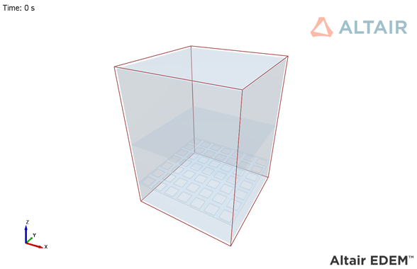
Define the Bulk Materials and Equipment Material
In this step, you will define the material models for the bar and sphere-shaped particles.
- In the Creator Tree, right-click Bulk Material and select Add Bulk Material.
- Rename the material to bar.
- In the Creator Tree, set the Solids Density property to 200 kg/m3 and the Shear Modulus to 1e7 Pa.
-
Click
 below Interaction to define the
interaction properties for collisions among the bar shaped particles. In the
dialog, click OK.
below Interaction to define the
interaction properties for collisions among the bar shaped particles. In the
dialog, click OK.
-
Set the interaction coefficients as shown in the figure below.
Figure 4. 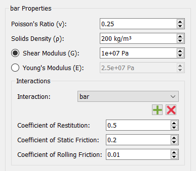
- In the Creator Tree, right-click bar and select .
- Rename the particle to bar.
- Under bar, click Properties.
-
In the bar Spheres panel, set the Physical Radius and the XYZ positions as
shown in the figure below.
Figure 5. 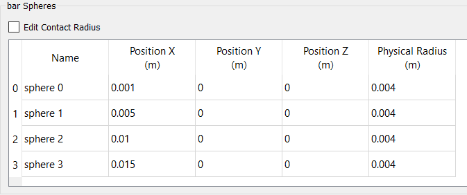
Note: When defining non-spherical shapes, you need to make sure that the principal axis of the particle is aligned with the x-axis, as shown in the figure below. The principal axis definition for some standard shapes is explained later in this tutorial.Figure 6. 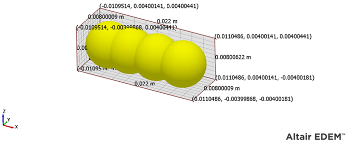
-
In the Creator Tree, click Calculate Properties.
Figure 7. 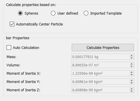
Note: Since the "Automatically Center Particle" option is active, EDEM will internally adjust the positions of the spheres in the particle. Although you might see minor changes in the location of the spheres, the overall dimensions of the particle stay the same. - Right-click Bulk Material and select Add Bulk Material.
- Rename the material to sphere.
- Set the Solids Density property to 1500 kg/m3.
-
Click below Interaction to define the
interaction properties for collisions with sphere particles. In the dialog,
select sphere and then click OK.
-
Set the interaction coefficients as shown in the figure below.
Figure 8. 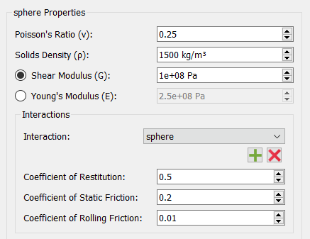
-
Click again to define the interaction
properties for collisions with bar particles. In the dialog, select
bar and then click OK.
-
Set the interaction coefficients as shown in the figure below.
Figure 9. 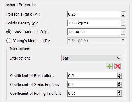
- In the Creator Tree, right-click sphere and select .
- Rename the particle to sphere.
- Under bar, click Properties.
-
In the sphere Spheres panel, set the Physical Radius of the sphere to
0.004 m and then press Enter.
Figure 10. 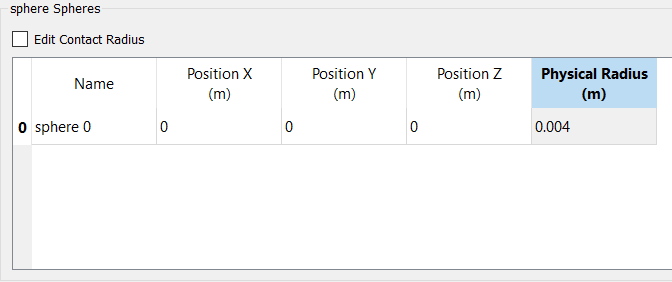
-
In the Creator Tree, click Calculate Properties.
Figure 11. 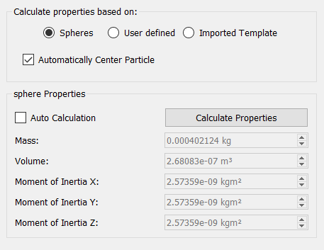
- Right-click Equipment Material and select Add Equipment Material.
- Rename the material to Steel.
- Set the Solids Density property to 7800 kg/m3.
-
Click below Interaction to define the
interaction properties for collisions with bar particles. In the dialog, select
bar and then click OK.
-
Set the interaction coefficients as shown in the figure below.
Figure 12. 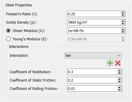
-
Click again to define the interaction
properties for collisions with sphere particles. In the dialog, select
sphere and then click OK.
-
Set the interaction coefficients as shown in the figure below.
Figure 13. 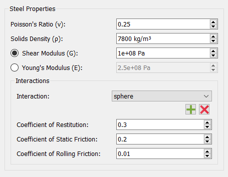
- Save the model.
Define Geometries and Factories
- In the Creator Tree, expand Geometries.
- Click Sieve and verify that the type is set to Physical.
- Right-click Sieve and select .
-
Name it oscillation and specify the parameters as shown
in the figure below.
Figure 14. 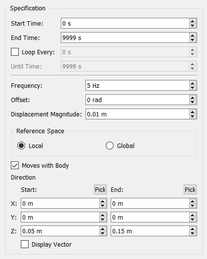
- Click Outlet and set the type to Virtual.
- Similarly, set the Inlet type to Virtual, the Walls type to Physical, and the Material type to Steel (if not set already).
- Click factory and set the type to Virtual
- Right-click factory and select Add Factory. Name it bar factory.
-
Set the particle generation parameters as shown in the figure below.
Figure 15. 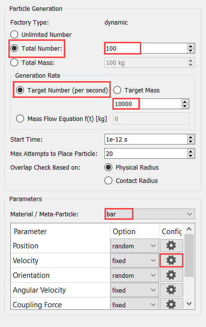
-
Click
 besides Velocity, set the
Z-velocity to -1 m/s, and then click OK.
besides Velocity, set the
Z-velocity to -1 m/s, and then click OK.
- Repeat steps 8-10 to create another factory named sphere factory. Use the same parameters but set the Total Number to 200 and the Material to sphere.
- Save the model.
Define the Environment
In this step, you will define the extents of the domain for the EDEM simulation and the direction of gravitational acceleration.
- In the Creator Tree, click Environment.
-
Activate the checkbox for Auto Update from Geometry (if
not already selected).
When a moving particle touches the bounding faces of the domain (environment), it will be removed from the simulation.
- Activate Gravity and set the z-value to -9.81 m/s2.
- Save the EDEM deck.
Define the Simulation Settings
-
Click
 in the top-left corner to go to
the EDEM Simulator tab.
in the top-left corner to go to
the EDEM Simulator tab.
-
In the Simulator Settings tab, set the Time Integration scheme to
Euler and de-activate the Auto Time
Step checkbox.
Note: The Auto time step should never be used for AS-EDEM bidirectional coupled simulations.
-
Set the Fixed Time Step to 1e-5 s.
Note: Generally, a value of 20-40% of the Rayleigh Time Step is recommended as the time step size to ensure stability of the DEM simulation. When setting the time step for the DEM model, make sure that the CFD time step is an integer multiple of DEM time step. In this case, the CFD time step is 1e-3, which is 50 times the DEM time step. This ensures that the physical time in both the solvers match at the end of each data exchange interval. Also, the recommended range for the CFD-to-DEM time step ratio is 50-200 for most cases.
- Set the Total Time to 1 s and the Target Save Interval to 0.01 s.
-
Set the Cell Size to 2.5 R min.
Generally, a value in the range of 2-6 Rmin is recommended as the optimum cell size.
-
Set the Selected Engine to CPU Solver and set the Number
of CPU Cores based on availability.
Figure 16. 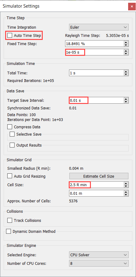
- Once the simulation settings have been defined, save the model.
Part 2 - AcuSolve Simulation
Start HyperMesh CFD and Open the HyperMesh Database
- Start HyperMesh CFD from the Windows Start menu by clicking .
-
From the Home tools, Files tool group, click the Open Model tool.
Figure 17. 
The Open File dialog opens. - Browse to the directory where you saved the model file. Select the HyperMesh file ACU-T6104_sieve.hm and click Open.
- Click .
-
Save the database as sieve_nonspherical in
the same directory as the other input files.
This will be the working directory and all the files related to the simulation will be stored in this location.
Validate the Geometry
The Validate tool scans through the entire model, performs checks on the surfaces and solids, and flags any defects in the geometry, such as free edges, closed shells, intersections, duplicates, and slivers.
Set Up Flow
Set the General Simulation Parameters
-
From the Flow ribbon, click the Physics tool.
Figure 19. 
The Setup dialog opens. - Under the Physics models setting, select the Multiphase flow radio button.
- Change the Multifluid type to Bidirectional EDEM Coupling.
-
Click the Eulerian material drop-down menu and select Material
Library from the list.
You can create new material models in the Material Library.
-
In the Material Library dialog, select EDEM 2
Way Multiphase, switch to the My Material
tab, and then click
 to add a new material model.
- In the microdialog, click EDEM Bidirectional Material in the top-left corner and change the name to Air-Particle.
- Set the Carrier field to Air (if not set already).
- Set the particle shape to Non-Spherical.
- Set the drag model to Rong.
-
Set the Non spherical drag coefficient model to
Holzer-Sommerfeld.
Figure 20. 
- Click the table icon beside the drag coefficient model drop-down.
-
In the new dialog, click
 to add a new row, and then enter the values for Aspect Ratio and Volume as shown
in the figure below.
to add a new row, and then enter the values for Aspect Ratio and Volume as shown
in the figure below.
Figure 21. 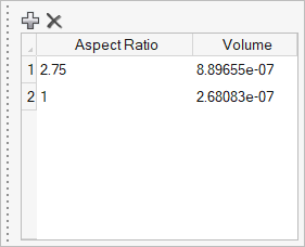
Note: The volumes entered here should be obtained from EDEM under particle properties. There might be slight variation in the volume values that you may see in your EDEM model but that is fine.Here the aspect ratios are calculated based on the ratio of the length to diameter of the particles. The AR of 2.75 and 1 are for bar and sphere-shaped particles respectively. The volume of the particles can be obtained from EDEM under the particle properties. If the simulation has particles of a single shape, then the volume field can be set to zero.
The image below explains the aspect ratio definition for some standard non-spherical particle shapes.Figure 22. 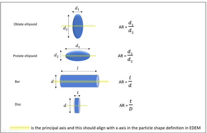
- Press Esc to close the dialog and then close the material model and Material Library dialogs as well.
- In the Setup dialog, set the Eulerian Material to Air-Particle.
- Set Time step size and Final time to 0.005 and 1, respectively. Select Spalart-Allmaras for the Turbulence model.
- Verify that Gravity is set to 0, 0, -9.81.
-
Set the Pressure scale to Absolute.
Figure 23. 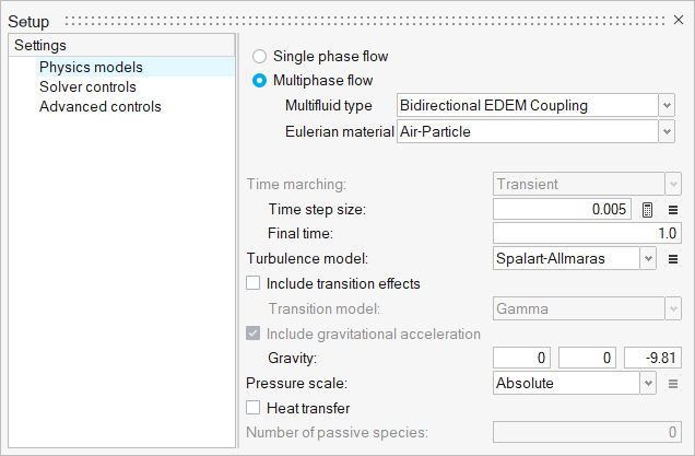
-
Click the Solver controls setting and set the Maximum
stagger iterations to 3.
Figure 24. 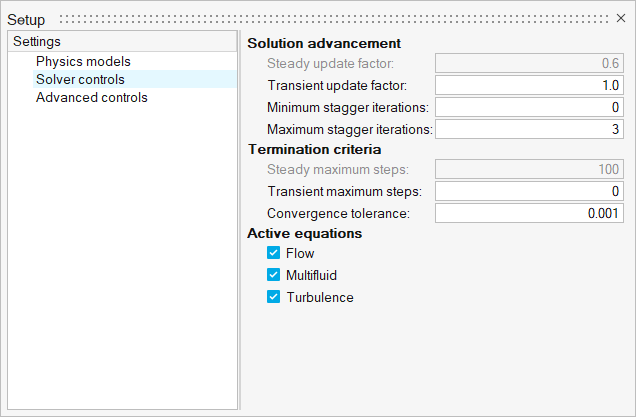
- Close the dialog and save the model.
Assign Material Properties
-
From the Flow ribbon, click the Material tool.
Figure 25. 
- Verify that Air-Particle has been assigned as the material.
-
On the guide bar, click
 to exit
the tool.
to exit
the tool.
Define Flow Boundary Conditions
-
From the Flow ribbon, Profiled
tool group, click the Profiled Inlet tool.
Figure 26. 
-
Click the inlet face highlighted in the figure below. In the microdialog, enter a value of 6 m/s
for the Average velocity and 1.0 for the Carrier fluid
volume fraction.
Figure 27. 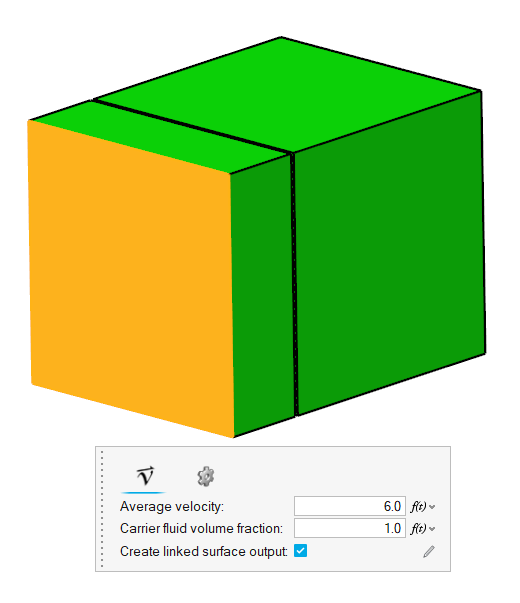
-
On the guide bar, click
 to execute
the command and exit the tool.
to execute
the command and exit the tool.
-
Click the Outlet tool.
Figure 28. 
-
Select the face highlighted in the figure below and then click on the
guide bar.
Figure 29. 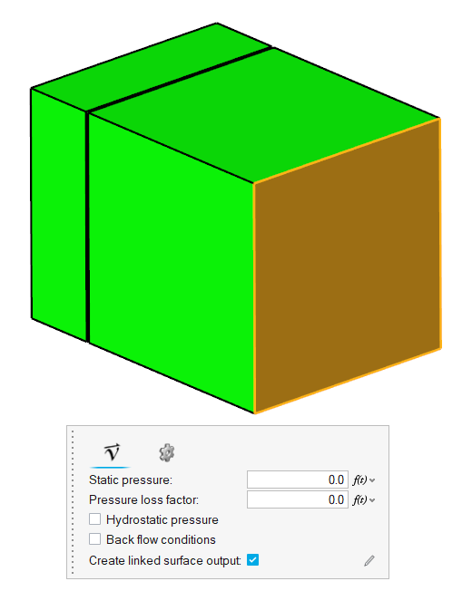
- Save the model.
Set Up Motion
Select the Motion Type
-
From the Motion ribbon, click the Settings tool.
Figure 30.
- In the Setup dialog, set the Mesh motion to Arbitrary and close the dialog.
Define the Mesh Boundary Conditions
-
From the Motion ribbon, click the Planar Slip tool.
Figure 31. 
-
Select the two surfaces highlighted in the figure below.
The surfaces selected have the minimum y-coordinate.
Figure 32. 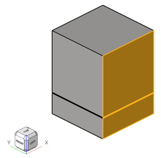
- In the Mesh Motion legend, double-click Planar Slip and change the name to y_neg.
-
On the guide bar, click
 to execute the command and remain in the
tool.
to execute the command and remain in the
tool.
-
Repeat steps 2-4 to create three more planar slip boundary conditions for the
surfaces with the maximum y-coordinates, and the minimum and maximum
x-coordinates. Name these groups y_pos,
x_neg, and x_pos
respectively.
Once the four planar slip conditions are defined, the Mesh Motion legend should look like the one shown below.
Figure 33. 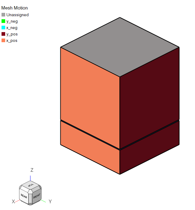
- Save the model.
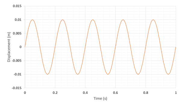
Define Sinusoidal Translational Motion
-
From the Motion ribbon, click the Translation tool.
Figure 34. 
- In the Mesh Motion legend, right-click Unassigned and select Isolate.
- On the guide bar, change the active selector to Surfaces.
-
Using box selection, select all the sieve surfaces as shown in the figure
below.
Ensure that you are not selecting the inlet or outlet faces.
Figure 35. 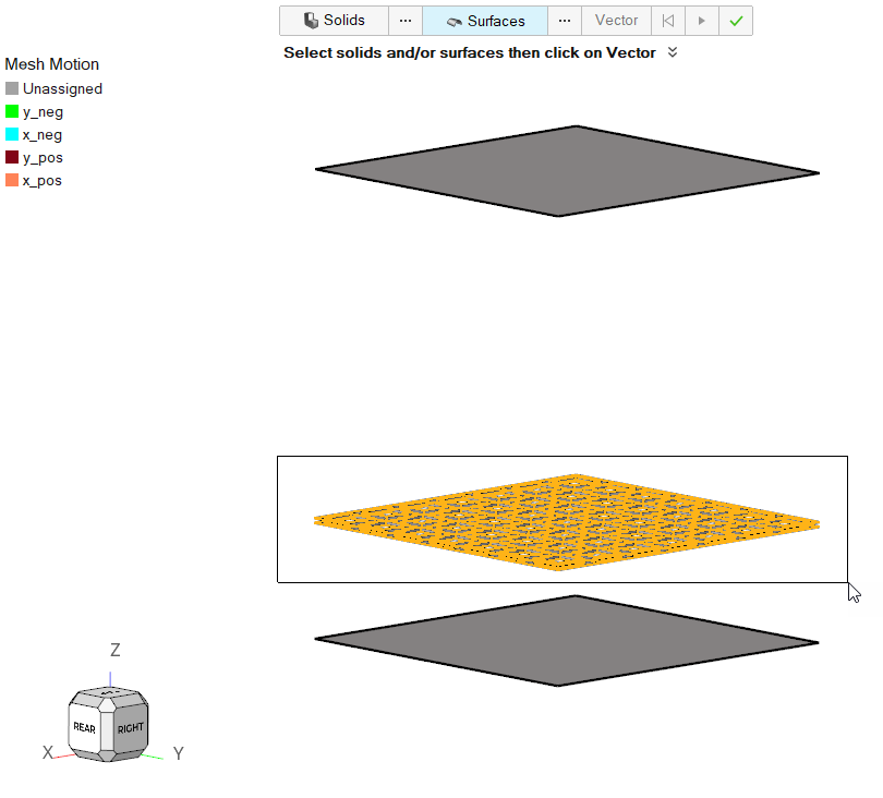
- Click Vector on the guide bar.
- Click anywhere on the sieve surfaces in the modeling window.
-
In the microdialog, click Z to
align the axis to the global z axis.
Figure 36. 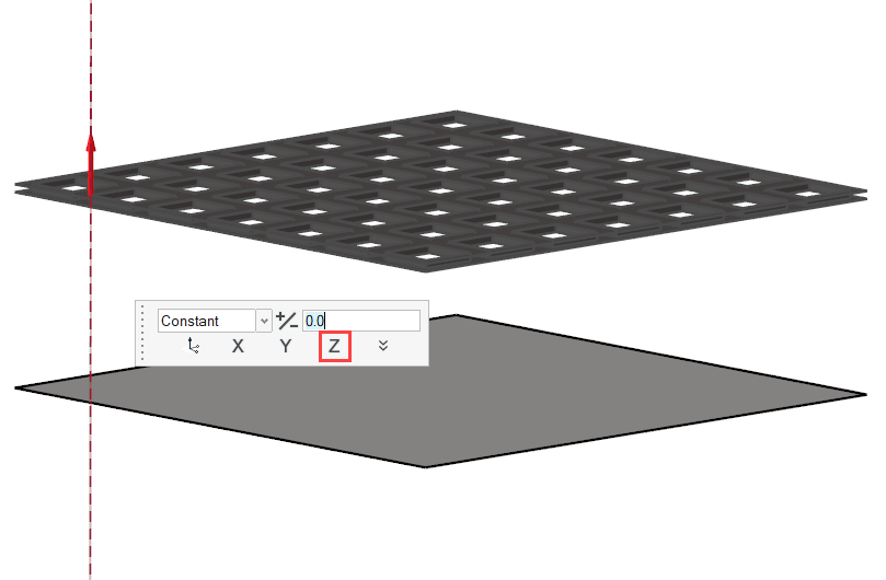
-
In the microdialog, change the type to
Time-varying and click the plot icon.
Figure 37. 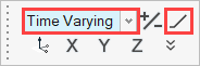
-
In the new plot dialog, click the drop-down beside the table icon for function
specification and select the oscillating option.
Figure 38. 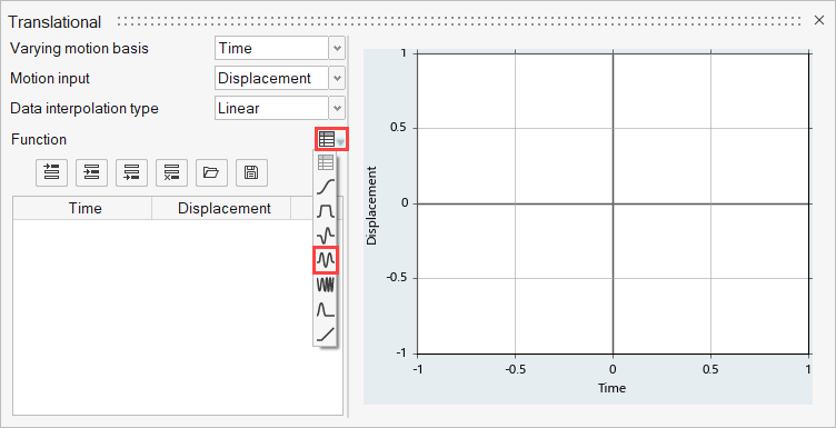
-
Enter the values for the sine function as shown in the figure below.
Figure 39. 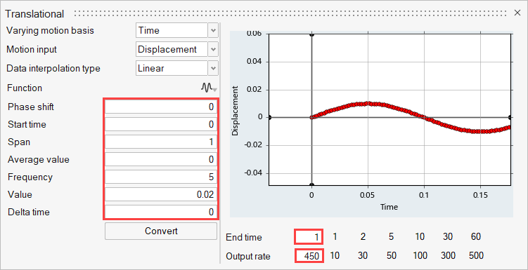
-
Click Convert to transform the sine function into an
array for the multiplier function.
The motion profile for the translation motion should look like the one shown below.
Figure 40. 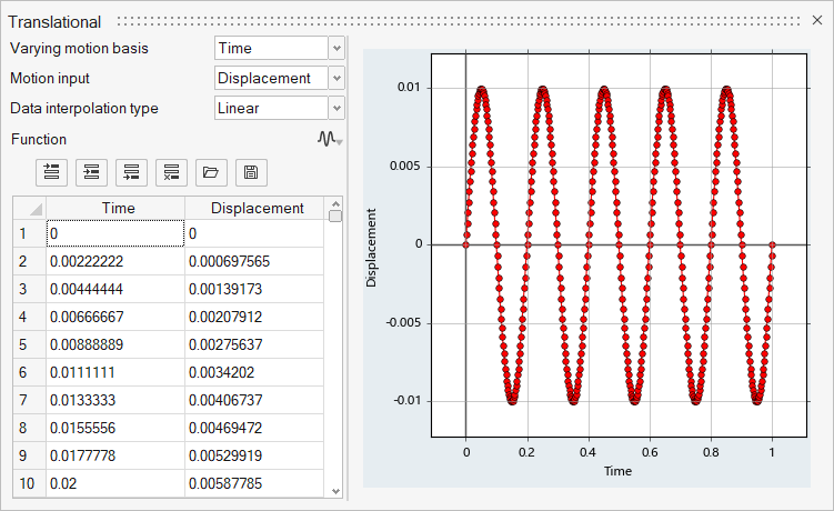
-
Click on the guide bar.
Generate the Mesh
-
From the Mesh ribbon, click the
Volume tool.
Figure 41. 
The Meshing Operations dialog opens. -
Set the Mesh size to Maximum size and change the Maximum
element size to 0.03.
Figure 42. 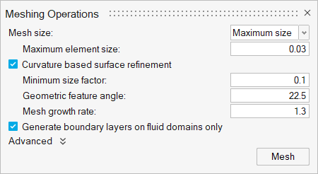
-
Click Mesh.
The Run Status dialog opens. Once the run is complete, the status is updated and you can close the dialog.Tip: Right-click the mesh job and select View log file to view a summary of the meshing process.
- Save the model.
Define Nodal Outputs
Once the meshing is complete, you are automatically taken to the Solution ribbon.
-
From the Solution ribbon, click the Field tool.
Figure 43. 
The Field Output dialog opens. - Check the box for Write Initial Conditions.
- Uncheck the box for Write results at time step interval
- Check the box for Write results at time interval.
-
Set the Time step interval to 0.05.
Figure 44. 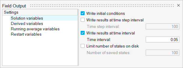
Submit the Coupled Simulation
-
Start the coupling server by clicking Coupling Server in
EDEM.
Figure 45. 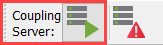
Once the Coupling server is activated, the icon changes.Figure 46. 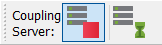
- Return to HyperMesh CFD.
-
From the Solution ribbon, click the Run tool.
Figure 47. 
The Launch AcuSolve dialog opens. - Set the Parallel processing option to Intel MPI.
- Optional: Set the number of processors to 4 or 8 based on availability.
- Expand Default initial conditions, uncheck Pre-compute flow and set the z-velocity value to 6. Uncheck Pre-compute Turbulence.
-
Click Run to launch AcuSolve.
Figure 48. 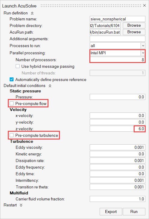
Once the AcuSolve run is launched, the Run Status dialog opens. -
In the dialog, right-click the AcuSolve run and
select View log file.
If the coupling with EDEM is successful, that information is printed in the .log file.
Figure 49. 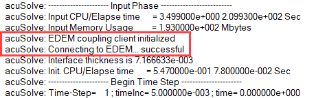
Once the simulation is complete, the summary of the run time is printed at the end of the .log file.Figure 50. 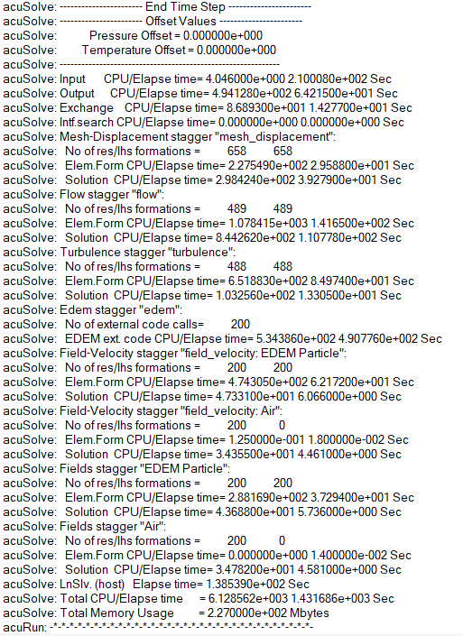
Analyze the Results
AcuSolve Post-Processing
-
In HyperMesh CFD, right-click the AcuSolve run in the Run Status
dialog and select Visualize results.
Figure 51. 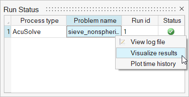
The results are loaded in the Post ribbon. -
Click the Slice Planes tool.
Figure 52. 
-
Select the x-z plane as highlighted in the figure below.
Figure 53. 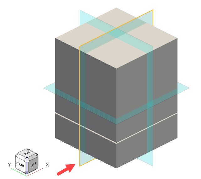
-
In the slice plane microdialog, click
 to
create the slice plane.
to
create the slice plane.
- In the display properties microdialog, set the display to velocity and activate the Legend toggle.
- Change the bounds of the legend to 0 and 15.
-
Click
 and set the Colormap name to Rainbow
Uniform.
and set the Colormap name to Rainbow
Uniform.
Figure 54. 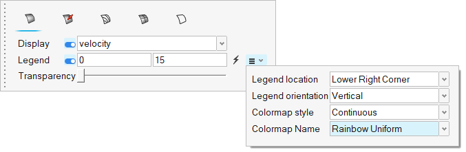
-
Click on the guide bar.
-
In the Post Browser, turn off the visibility of
Flow Boundaries by clicking its icon.
Figure 55. 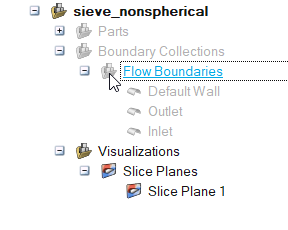
-
Select the Left face on the view cube to align the model
to the x-z plane.
Figure 56. 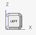
-
Click
 on the animation toolbar to view the animation of
the velocity contour.
on the animation toolbar to view the animation of
the velocity contour.
Figure 57. 
EDEM Post-Processing
-
Once the EDEM simulation is complete, click
 in the top-left corner to go to
the EDEM Analyst tab.
in the top-left corner to go to
the EDEM Analyst tab.
- In the Analyst Tree, expand and then select all geometries by holding the Ctrl key.
-
Verify that the Display Mode is set to Filled and set
the Opacity to 0.2.
Figure 58. 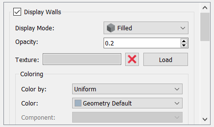
- In the Analyst Tree, click Particles.
- Set the coloring to Velocity.
- Activate the Auto Update checkboxes for both the Min and Max Value.
- Activate the Show Legend checkbox.
-
Click Apply All.
Figure 59. 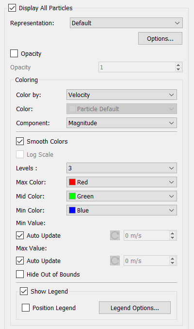
-
On the menu bar, set the time to
0 by clicking:
Figure 60. 
-
Set the View plane to + Y.
Figure 61. 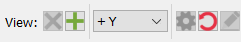
-
In the Viewer window, set the Playback Speed to 0.1x and
then click
 to play the particle flow animation.
Figure 62. 
Observe that the lighter bar shaped particles are blown away by the incoming fluid while the heavier particles fall through the sieve openings.
Summary
In this tutorial, you learned how to set up and run a basic AcuSolve-EDEM bidirectional (two-way) coupling problem with non-spherical particles. You learned how to create a non-spherical particle in EDEM and set up the AcuSolve model to consider the effect of the particle shape for the fluid-particle interaction forces. Once the simulation was complete, you learned how to post-process the AcuSolve results using HyperMesh CFD and the EDEM results.