ACU-T: 6106 AcuSolve - EDEM Bidirectional Coupling with Mass Transfer
Tutorial Level: Intermediate
Prerequisites
This tutorial introduces you to the workflow for setting up and running a basic
AcuSolve-EDEM
bidirectional coupling simulation with mass transfer. Prior to starting
this tutorial, you should have already run through the introductory tutorial,
ACU-T: 1000 Basic Flow Set Up and ACU-T: 6100 Particle Separation in a Windshifter using Altair EDEM, and have a basic understanding of
HyperMesh CFD, AcuSolve, and
EDEM. To run this simulation, you will need access
to a licensed version of HyperMesh CFD, AcuSolve, and EDEM.
Before you begin, copy the file(s) used in this tutorial to your working directory
and unzip the files.
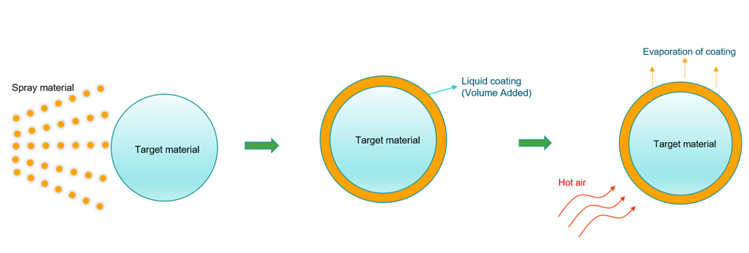
The spray coating update physics models allows you to simulate the coating process in
which the volume of a ‘spray’ particle is transferred to a target particle upon
contact. In this tutorial, a tablet coating process is simulated, in which spray
particles are sprayed onto a row of tablets. The spray particles are modeled as
solid particles in EDEM, and their properties are set to
that of water. When a spray particle touches the tablet, the volume of spray
particle is transferred to the tablet and the amount of coating is registered as a
custom property called ‘Volume Added’.Figure 1.
In a typical tablet coater, hot air is injected during the coating process. This
allows for the solvent to be evaporated and the solid content of the coating gets
deposited on the surface of the tablet. By coupling the spray coating model with the
heat and mass transfer models in AcuSolve, you can
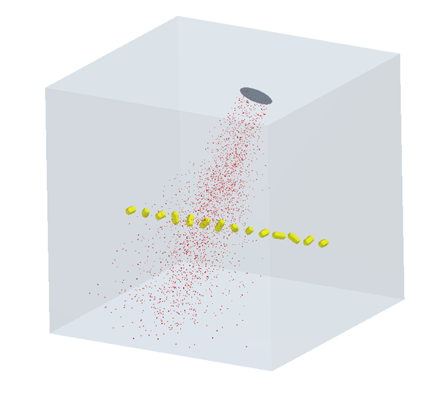
simulate the drying process as well. In this tutorial, the initial temperature of
the air is set to 363 K and the walls are considered as adiabatic. The tablet
particles are created with an initial temperature of 350 K. The spray particles are
injected for the first 0.25 s of the simulation and then the coating is left to
evaporate. In addition to the Volume Added (coating volume), the evaporation rate on
each particle can also be monitored.Figure 2.
Some assumptions of the spray coating model:
There is no momentum exchange between the spray material and the target
material or the geometry. Although, there is momentum exchange between the
spray particles and the carrier gas.
The spray particles do not exchange thermal energy with the carrier gas or
other particles/geometries.
The coating on a target particle is assumed to be transferred
instantaneously and uniformly across the surface of the particle.
The spray particles do not interact with each other. Hence, there is no
coalescence or breakup of spray droplets.
Part 1 - EDEM Simulation
Start Altair EDEM from the Windows start menu by clicking Start > Altair 2026 > EDEM 2026.
Open the EDEM Input Deck
From the menu bar, click File > Open.
In the dialog, browse to your problem directory and open the
tablet.dem file.
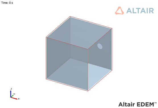
The geometry and the materials are loaded.Figure 3.
Review the Bulk Material and Particle Shape
Right-click in the Creator Tree and select Expand
All.
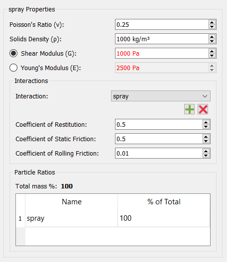
Under Bulk Material, click spray and verify that the
properties are set as shown below.
Figure 4.
Click Properties under spray. Verify that the particle
radius is set to 0.0001 m.
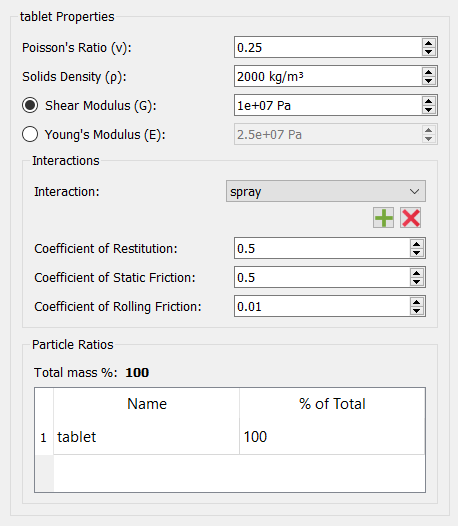
Click the tablet bulk material and verify that the
properties are set as shown below.
Figure 5.
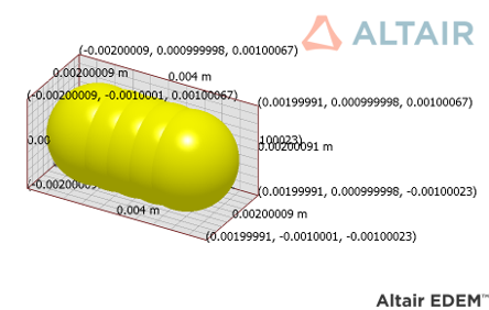
Click Properties under tablet and review the tablet
shape.
Figure 6.
The coordinate digit in the figure might be slightly different from those in
the database.
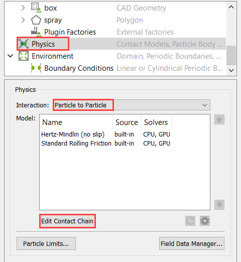
Set the Physics Models
In the Creator Tree, click Physics.
Set the Interaction to Particle to Particle and then
click Edit Contact Chain.
Figure 7.
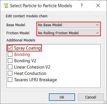
In the dialog, activate the checkbox for the Spray
Coating model. Set the Base and Friction models as shown in the
figure below and click OK.
The tutorial is set up in such a way that the tablet particles do not interact
with each other. Hence, the base contact models can be turned off for a faster
turnaround time.Figure 8.
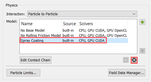
In the Creator Tree, select Spray Coating and then click
.
Figure 9.
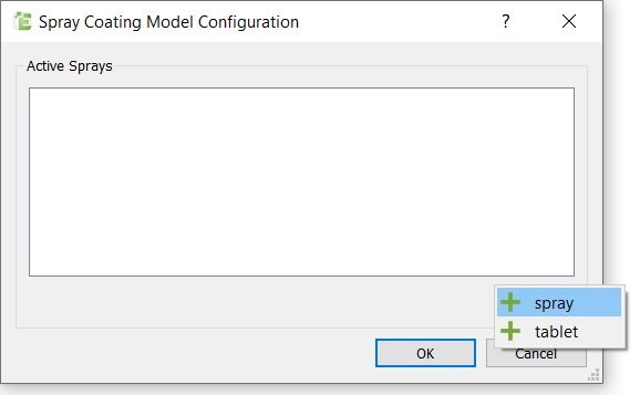
In the Spray Coating Model Configuration dialog, click
, select spray from the list
of materials, and then click OK.
Figure 10. The active spray material should be defined in both the ‘Particle to
Particle’ and ‘Particle to Geometry’ interactions to ensure that the simulations
stay stable even when the DEM time step is chosen based on the size of target
material.
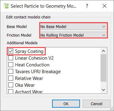
In the Creator Tree, change the interaction to Particle to
Geometry and then click Edit Contact
Chain.
In the dialog, set the same parameters as above and then click
OK.
Figure 11.
In the Creator Tree, select Spray Coating and then click
.
In the Spray Coating Model Configuration dialog, click
, select spray from the list
of materials, and then click OK.
Adding a material to the Particle to Geometry spray model will mean that when
a particle from this material contacts geometry, there will be no force applied
to the particle or geometry. This is important to stop unstable behavior when
running with a Time Step appropriate for the target material.
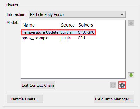
In the Creator Tree, change the interaction to Particle Body
Force and then click Edit Contact
Chain.
Note: In this simple example, the tablet particles are
created such that there are no tablet-tablet and tablet-geometry contacts.
Hence the contact models are turned off to save computational time. The
spray-tablet contacts are still active and are handled by the spray coating
physics model.
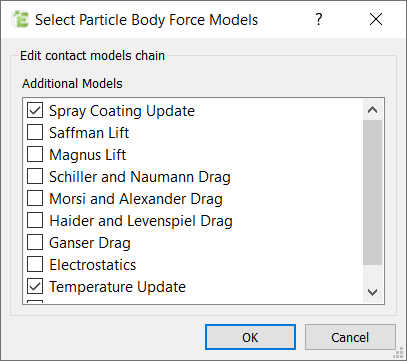
In the dialog, activate the checkboxes for Temperature
Update and Spray Coating Update and then
click OK.
Figure 12. By including the spray coating model in the particle body force, the
target material’s volume is updated. Without this, only the target material’s
Volume Added property will increase.
In the Creator Tree, select Temperature Update and then
click .
Figure 13.
Set the specific heat capacity of tablet and spray to
1200 and 4000 J/kg-K,
respectively, and then click OK.
Save the model.
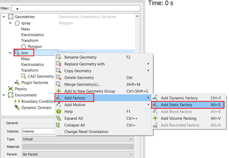
Define Geometries and Factories
Under Geometries, click box and verify that the type is
set to Virtual.
Right-click box and select Add Factory > Add Static Factory.
Figure 14.
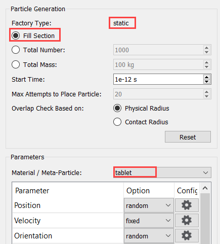
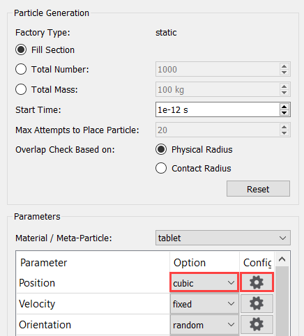
Set the particle generation parameters as shown in the figure below. Make sure
that the Material/Meta-Particle is set to tablet.
Figure 15.
Under Parameters, set the Position option to cubic and
then click .
Figure 16.
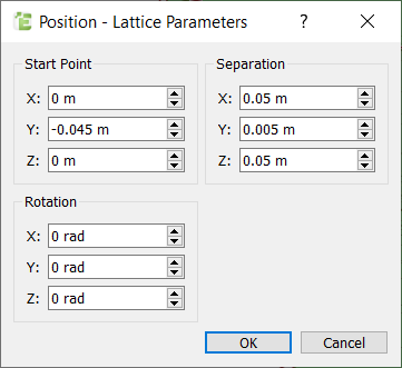
In the dialog, enter the position parameters as shown in the figure below and
then click OK.
This creates a row of tablet particles spaced evenly along the y-axis
and located at the center of the box.Figure 17.
Similarly, click next to the Temperature setting,
set the particle temperature to 350 K, and then click
OK.
Under Geometries, click spray and then change the type
to Virtual.
Right-click spray and select Add Factory > Add Dynamic Factory.
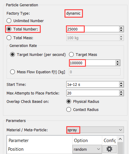
Set the particle generation parameters as shown in the figure below. Set the
Material to spray.
Figure 18.
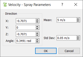
Under Parameters, set the Velocity option to spray and
then click .
In the dialog, set the spray velocity parameters as shown in the figure below
and then click OK.
Figure 19.
Similarly, click next to the Temperature setting,
set the particle temperature to 350 K, and then click
OK.
Save the model.
Define the Simulation Settings
Click in the top-left corner to go to
the EDEM Simulator tab.
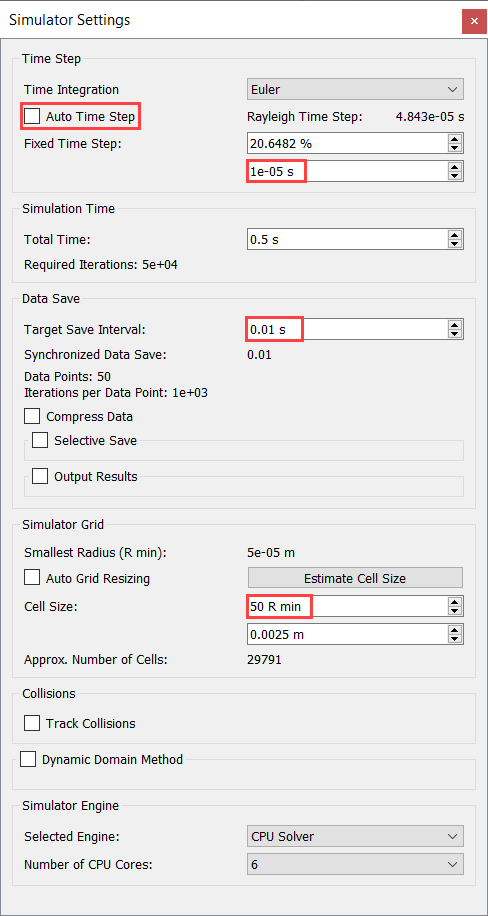
In the Simulator Settings tab, set the Time Integration scheme to
Euler and de-activate the Auto Time
Step checkbox.
Set the Fixed Time Step to 1e-5 s.
Note: Generally, a value of 20-40% of the Rayleigh Time
Step is recommended as the time step size to ensure stability of the DEM
simulation. Spray particles do not impart force on either geometry or any
other particles. This means you can run the simulation with the appropriate
time step for the target material.
Set the Total Time to 0.5 s and the Target Save Interval
to 0.01 s.
Set the Cell Size to 50 R min.
Set the Selected Engine to CPU Solver and set the Number
of CPU Cores based on availability.
Figure 20.
Once the simulation settings have been defined, save the model.
Part 2 - AcuSolve Simulation
Start HyperMesh CFD and Open the HyperMesh
Database
Start HyperMesh CFD from the Windows Start
menu by clicking Start > Altair <version> > HyperMesh CFD.
From the Home tools, Files tool group, click the Open Model tool.
Figure 21.
The Open File dialog opens.
Browse to the directory where you saved the model file.
Select the HyperMesh file ACU-T6106_tablet.hm and click
Open.
Validate the Geometry
The Validate tool scans through the entire model,
performs checks on the surfaces and solids, and flags any defects in the geometry,
such as free edges, closed shells, intersections, duplicates, and slivers.
To focus on the physics part of the simulation, this tutorial input file contains
geometry which has already been validated. Observe that a blue check mark appears on
the top-left corner of the Validate icon on the
Geometry ribbon. This indicates that the geometry is valid,
and you can go to the flow set up.Figure 22.
Set Up Flow
Set the General Simulation Parameters
From the Flow ribbon, click the Physics tool.
Figure 23.
The Setup dialog opens.
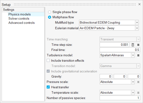
Under the Physics models setting, select the Multiphase
flow radio button.
Change the Multifluid type to Bidirectional EDEM
Coupling.
Set Time step size and Final time to 0.001 and
0.5, respectively. Select
Spalart-Allmaras for the Turbulence model.
Set the Pressure scale to Absolute.
Activate Heat transfer and set the Temperature scale to
Absolute.
Set the Number of passive species to 1.
This setting is necessary for the mass transfer feature to be active. The
evaporated moisture is tracked using the species transport equation.
Figure 24.
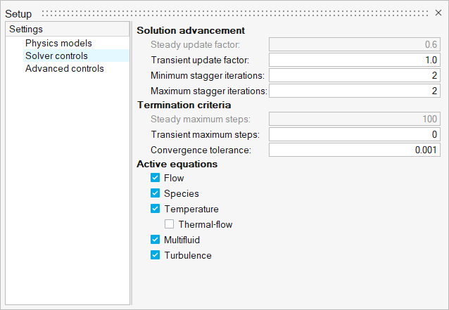
Click the Solver controls setting. Set the Minimum and
Maximum stagger iterations to 2 and
2, respectively.
Figure 25.
Close the dialog and save the model.
Assign Material Properties
From the Flow ribbon, click the Material tool.
Figure 26.
Verify that Air-EDEM Particle – 2way has been assigned as the material.
If not assigned, click the box geometry and select Air-EDEM
Particle – 2way from the microdialog.
On the guide bar, click to exit
the tool.
Since you are applying an adiabatic condition on the box walls, you don’t
need to set any thermal boundary condition explicitly.
Generate the Mesh
From the Mesh ribbon, click the
Volume tool.
Figure 27.
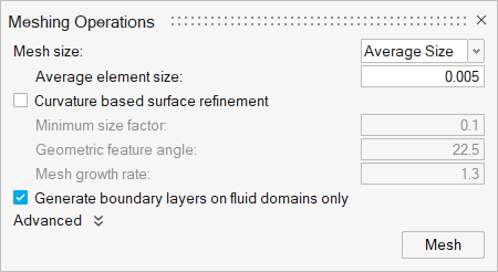
The Meshing Operations dialog opens.
Set the Mesh size to Average size and change the Maximum
element size to 0.005.
Deactivate Curvature-based surface refinement and then
click Mesh.
Figure 28.
Once the meshing process is complete, save the model.
Define Nodal Outputs
Once the meshing is complete, you are automatically taken to the Solution ribbon.
From the Solution ribbon, click the Field tool.
Figure 29.
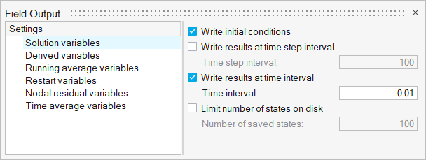
The Field Output dialog opens.
Check the box for Write initial conditions.
Uncheck the box for Write results at time step
interval
Check the box for Write results at time interval.
Set the Time step interval to 0.01.
Figure 30.
Close the dialog and save the model.
Submit the Coupled Simulation
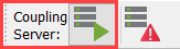
Start the coupling server by clicking Coupling Server in
EDEM.
Figure 31.
Once the Coupling server is activated, the icon changes.Figure 32.
Return to HyperMesh CFD.
From the Solution ribbon, click the Run tool.
Figure 33.
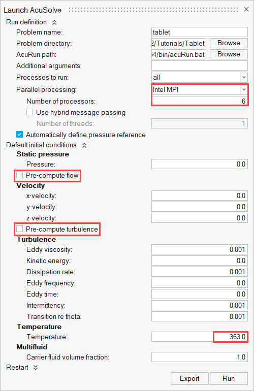
The Launch AcuSolve dialog opens.
Set the Parallel processing option to Intel MPI.
Set the Number of processors to 6.
Expand Default initial conditions, uncheck
Pre-compute flow and set the velocity values to
0. Uncheck Pre-compute
Turbulence.
Set the Temperature to 363 K.
Click Run to launch AcuSolve.
Figure 34.
Once the AcuSolve simulation is launched, it
connects with the EDEM coupling server. A warning
message is displayed indicating that the base contact models have not been set.
Click Ignore. Since the tablet particles are not in
contact with each other or with the geometry, you do not need any contact
models. The spray-tablet contacts are handled by the spray coating
model.
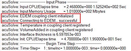
In the dialog, right-click the AcuSolve run and
select View log file.
If the coupling with EDEM is successful, that
information is printed in the .log file.Figure 35.
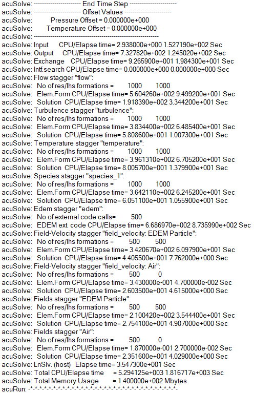
Once the simulation is complete, the summary of the run time is printed
at the end of the .log
file.Figure 36.
Post-Process the Results with EDEM
Once the EDEM simulation is complete, click in the top-left corner to go to
the EDEM Analyst tab.
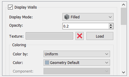
In the Analyst Tree, expand Display > Geometries and then select box.
Verify that the Display Mode is set to Filled and set
the Opacity to 0.2.
Figure 37.
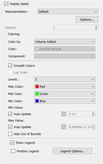
In the Analyst Tree, expand Particles and then click
tablet.
Set the coloring to Volume Added.
Activate the Auto Update checkbox for both Min and Max
Value.
Activate the Show Legend checkbox.
Figure 38.
On the menu bar, set the time to
0 by clicking:
Figure 39.
Set the View plane to Default.
Figure 40.
In the Viewer window, set the Playback Speed to 0.1x and
then click to play the particle flow animation.
Figure 41.
Observe that the added volume increases in the beginning as the tablets
receive the spray coating. Once the spray injection is stopped, the coating
starts to dry up and the added volume decreases gradually.
Summary
In this tutorial, you have learned how to set up and run a basic AcuSolve-EDEM bidirectional
(two-way) coupling problem with mass transfer. You learned how to create particles
with specific position and internal spacing and also learned how to define a spray
injection. Once the simulation was completed, you processed the results to view the
coating variation over time.

 .
.
 , select spray from the list
of materials, and then click OK.
, select spray from the list
of materials, and then click OK.
 in the top-left corner to go to
the EDEM Simulator tab.
in the top-left corner to go to
the EDEM Simulator tab.


 to exit
the tool.
to exit
the tool.


 in the top-left corner to go to
the EDEM Analyst tab.
in the top-left corner to go to
the EDEM Analyst tab.


 to play the particle flow animation.