Iron losses model
Introduction
- In the material
- In the post-processor, in Iron losses computation box
In both cases, the defined model is only used for the computation in the post-processor. Iron losses are not taken into account in the solving process.
In Flux, the iron losses models are only available on the laminated regions, the magnetic flux density used in these models is the homogenized magnetic flux density in a block of iron sheets defined by:

- : stacking factor
- : material magnetic flux density (iron, steel...)
- : air magnetic flux density
- : homogenized magnetic flux density
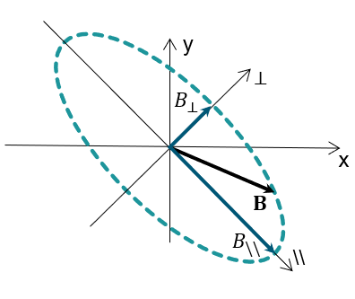
In the presence of rotating magnetic fields the curve By = f (Bx) can have an elliptical shape, thus it is more judicious to decompose homogenized induction vector of induction homogenize as follows:

- : magnetic induction in the longitudinal direction
- : magnetic induction in the transversal direction
Those both axis correspond to the minor and major axes of the elliptical curve described by the Figure 1.
Modified Bertotti model
Presentation of the model:
The theory of Bertotti gives us the expression of the magnetic losses depending on the frequency and the magnetic flux density.
The power density is expressed with this transient magnetic relation:


- : is the coefficient of losses by hysteresis
- : is the coefficient of classical Foucault currents losses
- : is the coefficient of supplementary losses or in excess*
- : is the exponent of losses by hysteresis
- : is the exponent of classical Foucault currents losses
- : is the exponent of supplementary losses or in excess*
- : frequency
- : homogenized magnetic induction
- : magnetic induction in the longitudinal direction
- : magnetic induction in the transversal direction
- : fill factor of the region
* the distinction between supplementary losses / in excess losses and classical losses is artificial. They can be grouped in one term and they therefore correspond to real induced currents flowing in the sheet.
A Compose tool designed for the identification of the modified Bertotti model coefficients from measurements is provided in Flux. Further information is available in the following user guide chapter: Material Identification.
Limits of validity
In a Steady state AC Magnetic application, power density is expressed with the following equation:

The software use the value of the magnetic flux density in each point. Consequently, it is convenient to be very careful with the results concerning the problems represented by the rotating machines with the Steady state AC Magnetic simulation. Indeed, for this type of simulation the rotor has a fixed position with respect to the stator, and the real rotor movement is modeled by changing the resistivity of the conductors of the rotor electric circuit. Thus, the calculated magnetic flux density is maximum in a point on the given position of the rotor in relationship with the stator, due to space harmonics. It follows that the calculated magnetic flux density does not correspond to the peak value of the magnetic flux density over a period in the time domain if the rotor were turning. Consequently, the computation of the magnetic losses must be utilized in this case with much caution.
Moreover, in the case of a non-linear approximation for the magnetic behavior law B(H), the saturation phenomenon, introduced by means of an equivalent model of magnetization, can alter the local values of the magnetic flux density.
Steps of the modified Bertotti model definition in the material
- Create material
- In Iron losses tab, check Model for iron losses computation and choose Modified Bertotti model
- Enter coefficients and exponents
LS model
Presentation:
- B(t) signal with common form and frequency
- Creation of a characteristic surface H(B, dB/dt) of the material measured experimentally.
- Reconstitution of H(t) signal (i.e. of the hysteresis cycle)
- Calculus of losses
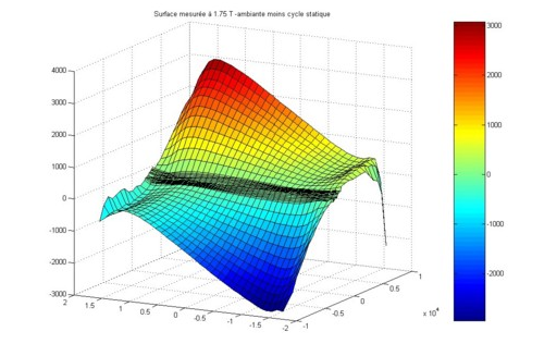
Characteristic surface H(B, dB/dt):
For each of the materials, the characteristic surface H(B,dB/dt) can be obtained by using a Epstein type device for magnetic measurements in medium frequency.
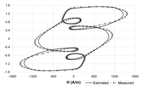
Reconstruction of the cycle:
An analytical model permits the reconstruction of H field from values of B:

The LS model is assigned to different nuances of laminations, which have been especially described to this purpose.
- NO 25
- M250-50A
- M270-35A
- M330-35A
- M330-65A
- M400-50A
- M600-50A
- M600-65A
- M800-50A
- M800-65A
For more informations about electrical steel sheets, see this page: Standards for electrical steel sheets
With this model, the user can also import his own materials in Flux (see LS model identification with MILS).
Definiton of the LS model in the material
See the section below: Isotropic soft material : Iron sheets described by LS model
- Additional information on iron loss with LS model is available in the following document: « Module LS pour l’estimation des pertes fer dans les machines électriques » - A. Lebouc – Rapport d’étude mai 2004