Magnetic losses (or iron losses) computation is a subsequent computation, carried out in Flux post-processor.
This chapter introduces iron losses computation, from modified Bertotti formulas, or with LS model (Loss Surface).
The power losses in electromechanical devices are mainly of three types:
the magnetic losses in the magnetic circuits (also called ‘iron losses’)
the losses by Joule effect in coils (also called ‘copper losses’)
the mechanical losses (mainly by friction in rotating machines)
Losses in magnetic materials:
The power losses in magnetic materials are connected to the phenomena associated with the time variation of the magnetic field. They are subdivided into hysteresis losses (of microscopic origin) and Foucault currents losses (of macroscopic origin). In fact, it is eddy current in both cases.
The hysteresis losses (microscopic eddy currents) are associated to currents
at a small scale. These currents are the result of local induction variation
caused by the magnetic structure in movement (essentially wall
movement).
The Foucault losses (macroscopic eddy currents) are due to the excitation
frequency. They appear when domain wall displacement increases due to
frequency increase.
Magnetic losses and hysteresis cycle:
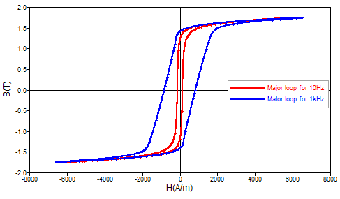
In practice, magnetic materials are characterized by their hysteresis cycle and the magnetic losses can be represented by this cycle, as presented below:
the volume energy created by hysteresis losses is corresponding to static hysteresis cycle (f<1Hz).
as the frequency increases, the cycle area increases and the volume energy created by eddy current losses is corresponding to the difference between the dynamic hysteresis cycle area and the static one.
Figure 1. Major cycles for different frequencies
Access to computation of iron losses
Iron losses computation can be accessed in Flux 2D, Skew and 3D for laminated regions
and for the following applications:
For modified Bertotti model: Steady state AC magnetic (averaged iron losses
computation) and transient magnetic (averaged or instantaneous iron losses
computation)
For LS model: Transient magnetic only (averaged or instantaneous iron losses
computation)
Note: * Laminated regions are often used in magnetic circuits of transformers
and of some electric machines in order to reduce eddy current losses.
Computation of iron losses
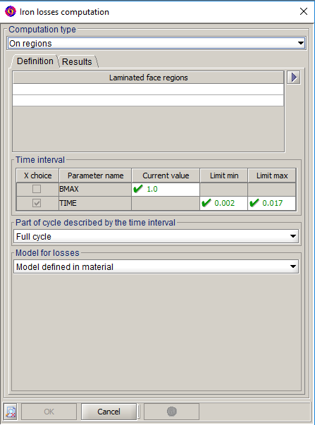
The computation box of iron losses can be accessed in the post-processing context via Computation > Computation of iron losses > Computation of iron losses
The box is as follows:
Computation type
The Computation type field enables to choose among the
following possibilities:
On regions : enables to compute modified Bertotti or
LS iron losses on a selection of laminated regions. The iron losses model
can be defined on the material or in this box via Model for
losses field. The computation gives instant losses and
averaged losses on the time interval for a set of fixed geometric parameters
or fixed I/O parameters.
Multi-parametric on regions : enables to compute
modified Bertotti or LS iron losses on a selection of laminated regions. The
iron losses model can be defined on the material or in this box via
Model for losses field. The computation gives
instantaneous losses for several sets of geometric parameters or I/O
parameters. This computation can be used in optimizations or efficiency
maps.
On point with LS model defined in the material: this
option can only be accessed in transient magnetic application. This calculus
enables to compute LS iron loss volume densities on a point in a laminated
region. Iron losses model must be defined in the material or the user can
also load his own losses file, see : LS model identification with MILS. The computation gives
instantaneous losses and averaged losses volume densities on the time period
for a set of fixed geometric parameters or I/O parameters. With this
computation, it is possible to display the hysteresis cycle.
Note: To ensure very fast computations of iron losses, Flux
needs to store - during the solving process - some data in .FLU folder and in
memory. This means that in case of scenarios with many parameter values (e.g.,
some thousands), the size of the .FLU folder and the required memory could grow
tremendously, thus limiting the performance of Flux for users who are not
interested in very fast iron losses computations. For such situations, the
option Data storage during solving exists in the Advanced tab of
the Solving process options dialog box accessible via the Solving
menu: it allows the user to disable the storage of data during solving and then
to reduce the size of the .FLU folder and the required memory. On the other
hand, the computations of iron losses slow down tremendously.
Note: In case of scenarios with geometric parameters, the data
storage for very fast iron losses computations is not allowed by Flux.
Consequently, the option described in the previous note has no effects.