Since version 2026, Flux 3D and Flux PEEC are no longer available.
Please use SimLab to create a new 3D project or to import an existing Flux 3D project.
Please use SimLab to create a new PEEC project (not possible to import an existing Flux PEEC project).
/!\ Documentation updates are in progress – some mentions of 3D may still appear.
Local quantities available for postprocessing
Introduction
The local quantities available for the postprocessing in the Steady State AC Electric application are stored in two categories:
- usual local quantities : the main characteristic quantities available in direct and easy access
- “advanced use” local quantities : the secondary quantities available in advanced use
Reminder
The fields of electric potential, electric field intensity, and electric flux density are time harmonic functions:
V(t) = V0ejωt
E(t) = E0ejωt
D(t) = [ε] E(t) ⇒ D(t) = E0ejωt = ([ε'] – j[ε "]) E0 ejωt
Usual local quantities
Usual local quantities available are presented on the table below.
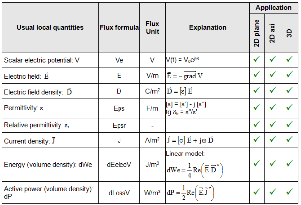
In D* and J*, the "*" means that it is the conjugate of the vector.
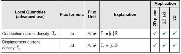
Advanced use
Usual local quantities available in advanced use are presented on the table below.