Since version 2026, Flux 3D and Flux PEEC are no longer available.
Please use SimLab to create a new 3D project or to import an existing Flux 3D project.
Please use SimLab to create a new PEEC project (not possible to import an existing Flux PEEC project).
/!\ Documentation updates are in progress – some mentions of 3D may still appear.
Flux e-Machine Toolbox: Input parameters
Introduction
After having opened the coupling component in Flux, the user must define several input parameters before running a test.
- Motor tab:
The parameters in this tab allow to:
- pilot the solving of the Flux project
- compute and build the different performance maps

- System tab:The parameters in this tab allow to:
- specify solving options (numerical memory, distribution, ...)

Input parameters - Motor tab: Wished data
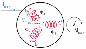
- Maximum phase current RMS
- Maximum phase voltage RMS
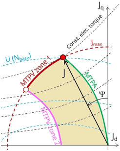
- Command mode:
- either MPTA: Maximum Torque Per Ampere
- either MTPV: Maximum Torque Per Volt
- Computation mode:
- either TM: Transient Magnetic solving
- either MS multi-positions: Magneto Static solving for multiple rotor positions
- either MS mono-position: Magneto Static solving for a single rotor position
- Maximum allowed rotating speed for the electrical machine
Input parameter - Motor tab: X Factor
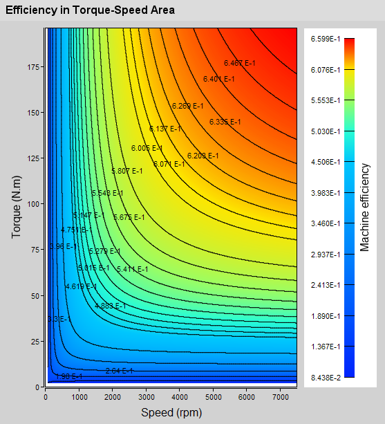
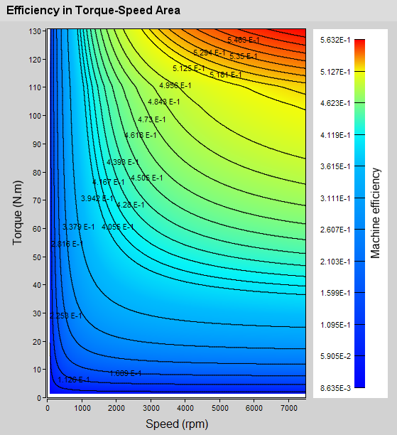
The X Factor allows the user to adjust the iron losses to his measurements and recompute the efficiency of his motor with a better accuracy. The X Factor is a floating value by which the iron losses amplitude is multiplied. The default value is 1.
The X Factor can be accessed:
- before solving: in the Input Parameters
- after solving: in Post-process with a New Command
- Iron Losses (Rotor + Stator) in Torque-Speed Area
- Rotor Iron Losses in Torque-Speed Area
- Stator Iron Losses in Torque-Speed Area
- Total Losses in Torque-Speed Area (including Iron Losses)
So with the MS mono-position computation mode, the X Factor is not available.
Input parameter - Motor tab: Torque computation mode
- Electromagnetic to compute the electromagnetic torque
- Useful to compute the useful torque, which
corresponds to the electromagnetic torque reduced by the torque loss due to
the iron losses:
Torque_useful = Torque_electromagnetic - (Iron_losses)/ω
where ω is the rotation pulsation in rad/s
| Electromagnetic mode | Useful mode |
|---|---|
 |
 |
- before solving: in the Input parameters
- after solving: in Post-process with a New Command
- For the torque computation, the Useful mode is only available with the TM and MS multi-positions computation modes (for which the iron losses are computed).
- With the MS mono-position computation mode, the iron losses are not computed, so the Useful mode is not available, the torque will therefore be computed with the Electromagnetic mode.
- From version 2023.1, with the TM and MS multi-positions computation modes, the default torque computation mode is the Useful mode.
- For all the tests run prior to version 2023.1, the torque was computed
with the Electromagnetic mode (this was the one
and only torque computation mode).
However, for the tests run with a version prior to 2023.1, with the MTPA and MTPV command modes, it is possible to rerun the torque computation with the Useful mode by using the button or the contextual menu Post-process with a New Command from version 2023.1.
Input parameters - Motor tab: Rotor initial angle
The Rotor initial angle is a necessary variable in order to apply Park’s transforms. Two possibilities:
- User: the user knows the initial angle of the rotor and can enter the value
- Auto: the value of the initial angle of the rotor is computed automatically. The goal is to find the rotor angle for t=0s in order to align it with the magnetic flux density in the airgap generated by the reference phase (e.g., phase A). Two simulations are performed in order to compute rotor initial angle. A path in the middle of the airgap is automatically defined in order to compute the magnetic flux density within it.
Input parameters - Motor tab: Number of computations requested
- With the TM computation mode:
- Number of computations for Jd and Jq (8 by default)
- Number of computations for the speed (10 by default)
- Number of computations per electrical period (30 by default)
Note: The total number of computations with the defaults values is 8*8*10*(30+3) = 21120 computations points. The 3 points on the electrical period are added to evaluate iron losses at both ends of the signal. It is necessary to have enough points to obtain a good Torque-Speed envelope. So the calculation time can therefore be quite long. The choice of values is a compromise between accuracy of results and solving time. The default values allow this compromise. - With the MS multi-positions computation mode:
- Number of computations for Jd and Jq (8 by default)
- Number of computations per electrical period (30 by default)
Note: For this MS multi-positions computation mode, it is not possible to modify the Number of computations for the speed. This field is disabled (grayed out). - With the MS mono-position computation mode:
- Number of computations for Jd and Jq (8 by default)
Note: For this MS mono-position computation mode:- The parametric solving process is done only on the parameters Jd and Jq.
- It is not possible to modify the Number of computations for the speed, nor the Number of computations per electrical period. These two fields are disabled (grayed out).
With this MS mono-position computation mode, the computation is faster than with the TM and MS multi-positions computation modes.
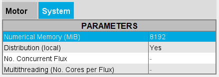
Input parameters - System tab: Numerical Memory
Numerical memory allocated to the solving process of the Flux project:
Since FeMT 2021, there is a new memory mode to run tests: the Dynamic memory mode.
From now on, there are two memory modes: User (static) and Dynamic.
- If the User (static) memory mode is used, then the
numerical memory value (in MiB) allocated to the solving process of the Flux
project is displayed. The user can modify this value.
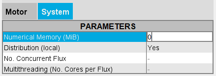
On the other hand, the user can switch to the Dynamic numerical memory mode by entering 0.
 Note: For FeMT versions prior to 2022.1, the user could not switch to the Dynamic memory mode in FeMT. In order to run tests in Dynamic memory mode, the user had to regenerate the coupling component from a Flux running in Dynamic memory mode.
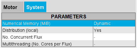
 - If the Dynamic memory mode is used, then
Dynamic is displayed and the numerical memory used is
dynamically managed by Flux during its execution. So in this mode, the user does
not set any value for the numerical memory.
On the other hand, the user can switch to the User numerical memory mode by entering a numerical value in MiB.
Warning: When switching from Dynamic numerical memory mode to User numerical memory mode, the user must know the numerical memory required to solve the project and therefore set a high enough value.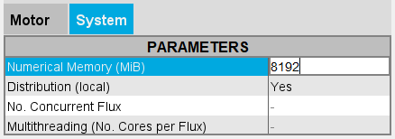
Note: For FeMT versions prior to 2022.1, the user could not switch to the User memory mode in FeMT. In order to run tests in User memory mode, the user had to regenerate the coupling component from a Flux running in User memory mode.
Input parameter - System tab: Distribution (local)
- If the Distribution (local) is set to
Yes
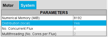
- If the distribution is activated in the Flux Supervisor that is to say that it has already been configured (Number of Concurrent Flux and Number of cores per concurrent Flux) and that you want to use distributed computing, then the solving will be distributed.
- If the distribution is not activated in the Flux Supervisor then the solving will be sequential and not distributed even if the Distribution (local) is set to Yes.
Note:- In order to activate the distribution in the Flux Supervisor:
- either use the Distribution Manager button
- or use the Options button and in System / Parallel computing, click on the Set local resources button
and possibly click on the Allow button and then define the local resources (Number of Concurrent Flux and Number of cores per concurrent Flux) and click on the Use button
- In order to deactivate the distribution in the Flux
Supervisor:
- either use the Distribution Manager button
- or use the Options button and in
System / Parallel
computing, click on the Set
local resources button
and possibly click on the Do Not Allow button or click on the Stop Using button
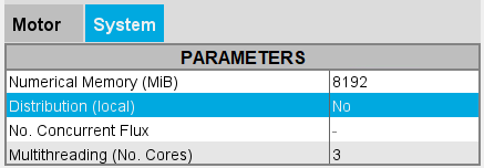
- If the Distribution (local) is set to
No then the solving will be sequential, not distributed.
For more information on distribution configuration, please see Parametric distribution with Flux
Input parameter - System tab: No. Concurrent Flux
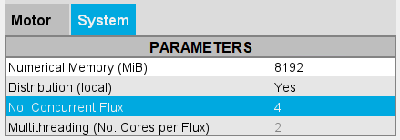
This field defines the number of Flux that can be running at the same time during a distributed computation.
This number of concurrent Flux is not accessible to the user here, it is grayed out.
- If the Distribution (local) is set to
Yes
- If in the field No. Concurrent Flux there
is a value n, then this indicates that
the distribution has already been configured i.e. that this
value has been previously set in the Flux Supervisor. So, for
the solving, n Flux will be run in parallel.Warning: A great number may render difficult the use of the machine for other tasks until the solving completes.
- If in the field No. Concurrent Flux there is no value, then this indicates that the distribution has not been activated in the Flux Supervisor. And so the solving will be sequential and not distributed even if the Distribution (local) is set to Yes.
Note:- In order to configure the distribution in the Flux Supervisor
and define the number of concurrent Flux:
- either use the Distribution Manager button
- or use the Options button and in System / Parallel computing, click on the Set local resources button
and possibly click on the Allow button and then define the Number of Concurrent Flux and click on the Use button
- In order to deactivate the distribution in the Flux
Supervisor:
- either use the Distribution Manager button
- or use the Options button and in System / Parallel computing, click on the Set local resources button
and possibly click on the Do Not Allow button or click on the Stop Using button
- If in the field No. Concurrent Flux there
is a value n, then this indicates that
the distribution has already been configured i.e. that this
value has been previously set in the Flux Supervisor. So, for
the solving, n Flux will be run in parallel.
- If the Distribution (local) is set to No then this field is not to be filled in, it will not be used as the solving will be sequential and not distributed.
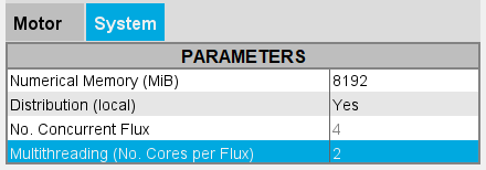
Input parameter - System tab: Multithreading (No. Cores)
This field defines the number of cores used during a solving. More precisely, it is the number of cores used by the application for multithreaded algorithms. The application uses at least 1 core.
- If the Distribution (local) is set to
Yes
- If in the field Multithreading (No. Cores per
Flux) there is a value m,
(note: this value is not accessible to the user here, it is
grayed out), then this indicates that the distribution has
already been configured i.e. that this value has been previously
set in the Flux Supervisor. So, for the solving,
m cores per concurrent Flux will be used.
- If in the field Multithreading (No. Cores per Flux) there is no value, then this indicates that the distribution has not been activated in the Flux Supervisor. And so the solving will be sequential and not distributed even if the Distribution (local) is set to Yes.
Note:- In order to configure the distribution in the Flux Supervisor
and define the number of cores per concurrent Flux:
- either use the Distribution Manager button
- or use the Options button and in System / Parallel computing, click on the Set local resources button
and possibly click on the Allow button and then define the Number of cores per concurrent Flux and click on the Use button
- In order to deactivate the distribution in the Flux
Supervisor:
- either use the Distribution Manager button
- or use the Options button and in System / Parallel computing, click on the Set local resources button
and possibly click on the Do Not Allow button or click on the Stop Using button
- If in the field Multithreading (No. Cores per
Flux) there is a value m,
(note: this value is not accessible to the user here, it is
grayed out), then this indicates that the distribution has
already been configured i.e. that this value has been previously
set in the Flux Supervisor. So, for the solving,
m cores per concurrent Flux will be used.
- If the Distribution (local) is set to
No then the solving will be sequential and not
distributed.
However, even if the solving is sequential, the number of cores will be used for multithreaded algorithms.

Default values are set for the field Multithreading (No. Cores):- For a 2D project, the number of cores is 1 by default
- For a Skew project, the number of cores is 2 by default
- For a 3D project, the number of cores is 4 by default
This value corresponding to the number of cores can be modified by the user. The maximum value the user can enter is of course the total number of cores of the machine.