Since version 2026, Flux 3D and Flux PEEC are no longer available.
Please use SimLab to create a new 3D project or to import an existing Flux 3D project.
Please use SimLab to create a new PEEC project (not possible to import an existing Flux PEEC project).
/!\ Documentation updates are in progress – some mentions of 3D may still appear.
Flux e-Machine Toolbox: About
Introduction

Starting from the 2019.1 version, Flux has a new tool called Flux e-Machine Toolbox. This coupling is available in 2D, 3D and Skew for the magnetic transient application.
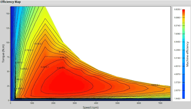
The aim of Flux e-Machine Toolbox is to characterize the behavior of the machine in the "Torque-Speed" area and allows to postprocess various quantities in this area.
Input parameters like the maximum phase voltage RMS , the maximum phase current RMS and the desired Maximum speed of the machine are considered.
Since FeMT 2024.1:
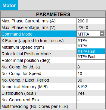
- MTPA: Maximum Torque Per Ampere
- MTPV: Maximum Torque Per Volt

The two command modes MTPA Fast and MTPV Fast have been removed.
But a new field has been created, entitled Computation mode.
-
TM: corresponds to the solving process called standard in the previous versions, i.e. the former MTPA and MTPV command modes.
This mode allows to compute the iron losses and the magnet losses.
The solving process is performed in Transient Magnetic.
The computation is more precise than with the MS computation modes (MS multi-positions and MS mono-position), but takes longer.
-
MS multi-positions: corresponds to a new solving process implemented in version 2025.
This new mode allows to compute the iron losses, but not the magnet losses.
The solving process is performed in Magneto Static, with a scenario dependent on the rotor position, i.e. for multiple rotor positions.
The computation is slightly less precise than in TM computation mode, but is faster.
-
MS mono-position: corresponds to the solving process called fast in the previous versions, i.e. the former MTPA Fast and MTPV Fast command modes.
This mode does not allow to compute the iron losses, nor the magnet losses.
The solving process is performed in Magneto Static for a single rotor position.
The computation is very fast.

| Before version 2024.1 | From version 2024.1 | |
|---|---|---|
| Command Mode | Command Mode | Computation Mode |
| MTPA | MTPA | TM |
| MTPA Fast | MTPA | MS mono-position |
| MTPV | MTPV | TM |
| MTPV Fast | MTPV | MS mono-position |
Type of machine
In these first versions, only one machine is taken into account by Flux e-Machine Toolbox. It is the Synchronous machine, permanent magnet in three phases (Inner rotor or outer rotor).
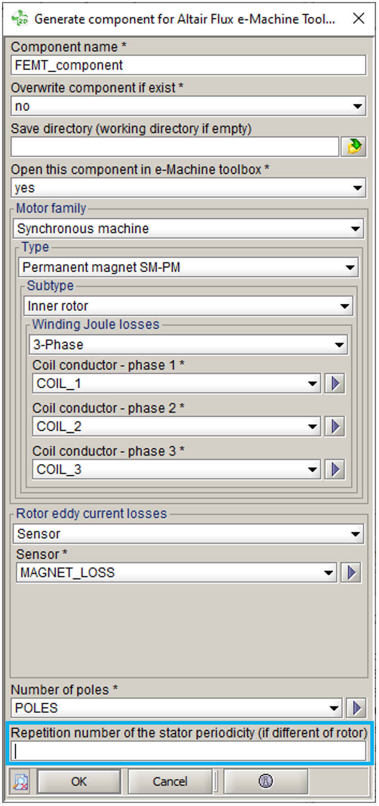
Since FeMT 2021, designs where the section represented in Flux contains multiple magnetic poles are supported. You can represent all types of machines, and in particular the fractional slot winding machines which have different periodicities in the stator winding and in the rotor.
In Flux, when generating the coupling component, there is a new field: Repetition number of the stator periodicity (if different of rotor)

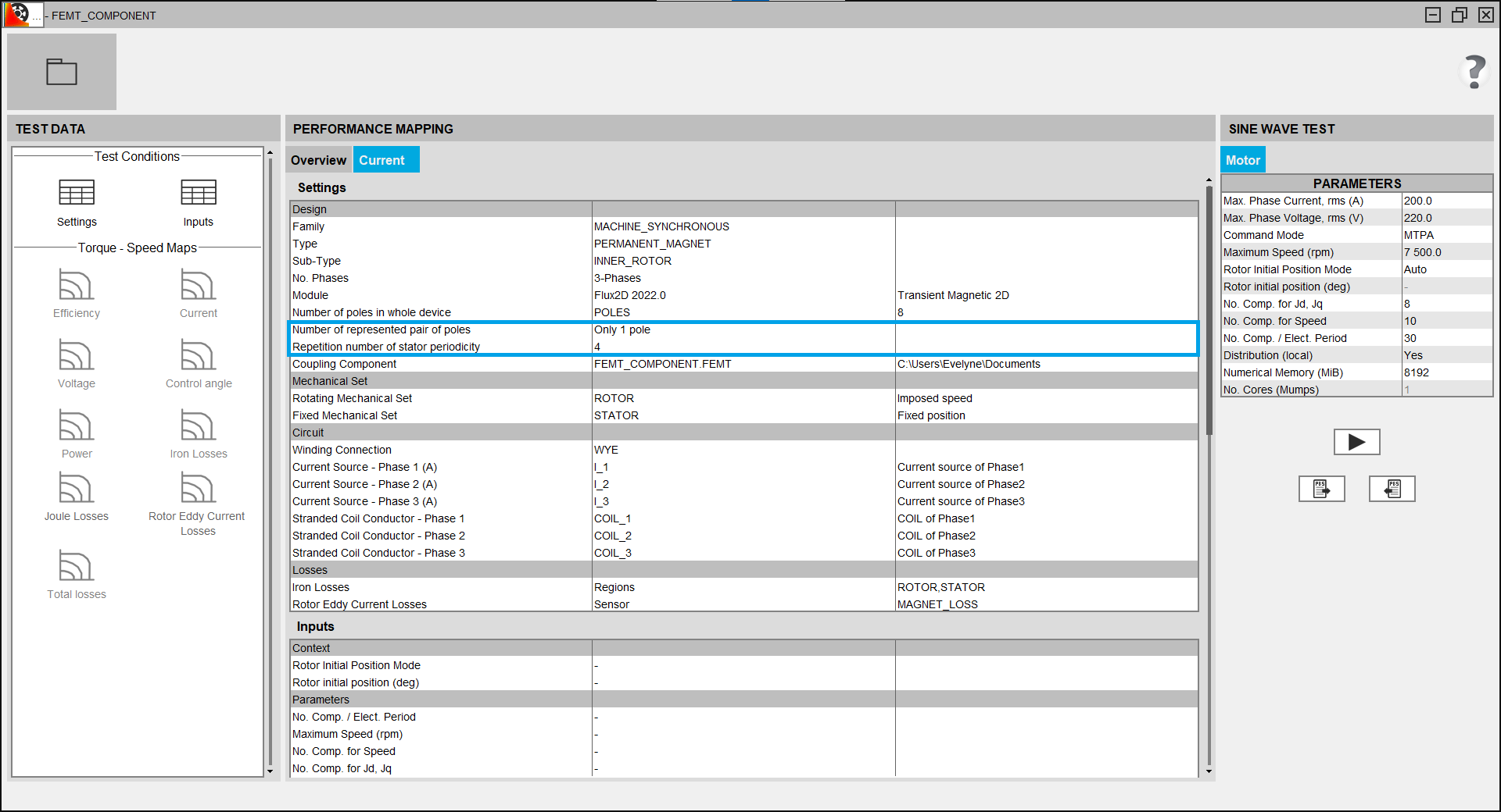
- Number of represented pair of poles
- Repetition number of stator periodicity

Type of circuit connection
WYE and DELTA winding connections are supported.
- On Flux side
When generating the component, the associated circuit is automatically analysed to know if it's a DELTA or a WYE connection.
-
On FeMt side
When opening the coupling component in Altair Flux e-Machine Toolbox, the winding connection is displayed in the settings table, in the Circuit section.
About losses
Different losses are computed and postprocessed:
- Stator Winding Joule Losses: on each coil conductor
- Rotor Eddy Current Losses: on solid conductor regions (magnet, fret, can,…)
- Iron losses:
- In 2D and 3D and in Skew since FeMT 2021:
- Only computed on non-conducting laminated magnetic regions
- In Flux, it is advised to choose a material with losses, assigned to these regions (the user has the choice to use LS or Bertotti model)
- If losses are not defined on the material, default Bertotti
coefficients are automatically applied
(K1=151.88 ; K2=0.07 ; K3=1.19 ; A1=2 ; A2=2 ; A3=1.5)
Note: For FeMT versions prior to 2021, for Skew projects:- Only computed on non-conducting magnetic regions , because the laminated regions did not exist in Skew
- Default Bertotti coefficients were automatically applied
after the Flux solving process
(K1=151.88 ; K2=0.07 ; K3=1.19 ; A1=2 ; A2=2 ; A3=1.5)
Note: About FeMT Skew coupling components generated from Flux version 2020.1 or older:FeMT 2021 no longer supports computation of iron losses for older Skew projects with no laminated regions.
However, the old Skew projects can be opened in FeMT 2021 and results of previous simulations computed with older FeMT version can be displayed. But, it is not possible to start a new simulation on this old project.
In order to run a new simulation on this old project, you will have to open your Skew project with Flux 2021 and regenerate a FeMT coupling component.
- In 2D and 3D and in Skew since FeMT 2021:
Iron losses computation strategy
With the TM and MS multi-positions computation modes, the iron losses are computed using an internal method called "Half cycle". This method allows to compute the iron losses over half an angular period, thus reduces the total number of computation steps and therefore improves performance by reducing computation time without altering the results.
Process
Here is the process of the Flux e-Machine Toolbox coupling:
| Step | Software | Description |
|---|---|---|
| 1 | Flux | Preparation of the Flux project:
Note: A classic workflow is to use FluxMotor to pre-design the
electrical machine and export it in a python srcipt. Then the
python script is run in Flux to obtain a Flux 2D project ready
to generate the coupling component |
| 2 | Flux | Generation of the Flux e-Machine Toolbox coupling component Note: In the options of the generation of the coupling
component, it is possible to choose to go directly at the
Step 5. After the generation of the coupling component, Flux
e-Machine Toolbox is launched (equal to step 3) and the
generated component is directly opened (equal to step
4)
|
| 3 | Flux Supervisor | Opening of Flux e-Machine Toolbox starting from Flux |
| 4 | e-Machine Toolbox | Opening of the Flux e-Machine Toolbox coupling component generated by Flux |
| 5 | e-Machine Toolbox | Choice of input parameters |
| 6 | e-Machine Toolbox | Launching of the simulation
Once the solving process is done, a postprocessing script is run to build the performance mapping |
| 7 | e-Machine Toolbox | Postprocessing of results |