Since version 2026, Flux 3D and Flux PEEC are no longer available.
Please use SimLab to create a new 3D project or to import an existing Flux 3D project.
Please use SimLab to create a new PEEC project (not possible to import an existing Flux PEEC project).
/!\ Documentation updates are in progress – some mentions of 3D may still appear.
Flux e-Machine Toolbox: Postprocessing
Introduction
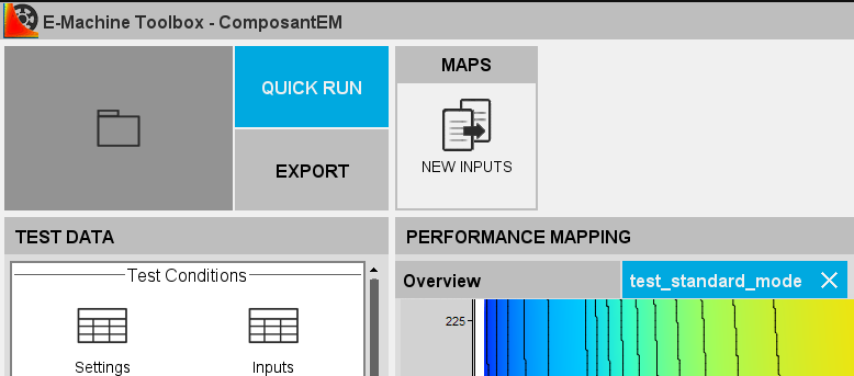
Once the test running is completed, performance maps are displayed in the central area. The filters on the left allow to display directly the performance map wished. The user has the possibility to use a cursor to display values by pointing on the map.
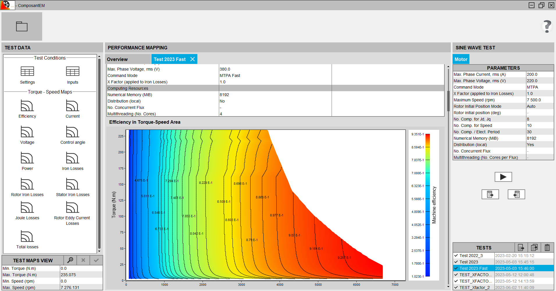
Performance maps
Several quantities are postprocessed in the Torque-Speed area:
- Efficiency
- Phase current
- Phase voltage
- Control angle
- Mechanical power
- Iron losses in rotor and stator
- Iron losses in rotor
- Iron losses in stator
- Stator winding Joule losses
- Rotor Eddy current losses
- Total losses: the sum of these 3 types of losses
- With the MS multi-positions computation mode, the eddy current losses are not computed. The corresponding map is therefore not available.
- With the MS mono-position computation mode, the iron losses and the eddy current losses are not computed. The two corresponding maps are therefore not available.
Efficiency map manipulations
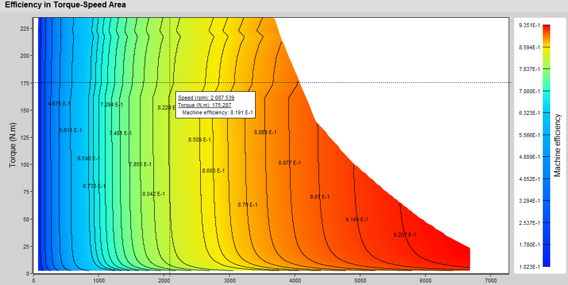
Cursor
The user can display efficiency map values at the cursor position.
Scale modification
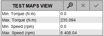
It is possible to modify the scales of all efficiency maps:
- graphically
- manually
- Click on

- On the efficiency map, do a rectangle selection
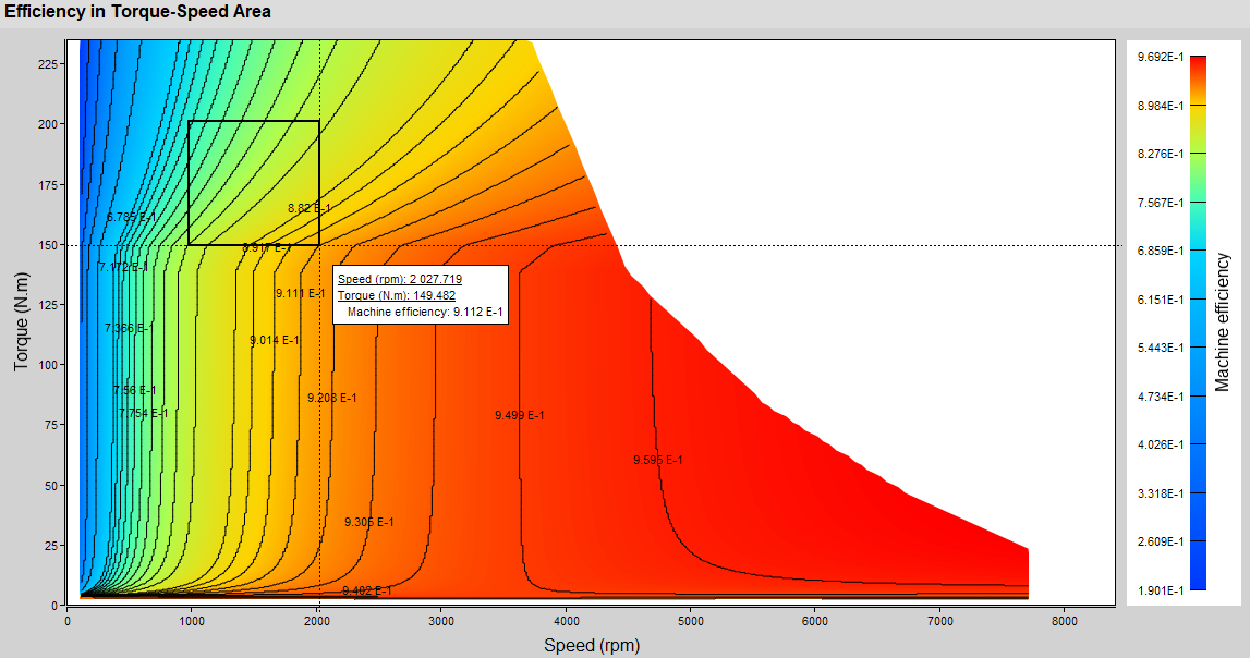
→ Map rebuilding takes a few seconds

→ Recomputed efficiency maps are updated
Before modification After modification 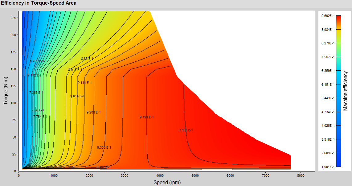
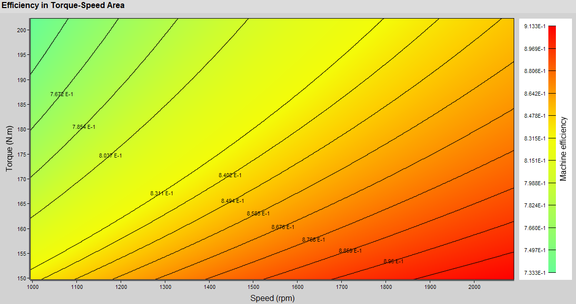
→ Values are updated
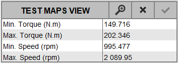
Steps for manual modification of scales
- Edit the value you want to modify
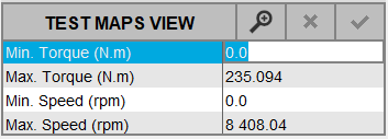
-
Modify the wished value and validate with the Enter key
-
Edit and Modify other values if you want
-
Validate all modifications by clicking on

→ Map rebuilding takes a few seconds
→ Recomputed efficiency maps are updated
Before modification After modification 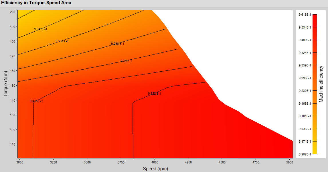

Skew specificity
In Flux, the description of a Skew model is done in the 2D environment. The 3D device is then rebuilt for the postprocessing. The face regions become volume regions.
Since FeMT 2021, for Skew projects, the iron losses are now computed on non-conducting laminated magnetic regions only.
- It is mandatory to use non-conducting laminated magnetic regions for the stator and the rotor.
- It is recommended to define a material with losses model and to assign it to non-conducting laminated magnetic regions (stator and rotor), otherwise default parameter values will be used for the iron loss computation.
The iron losses were only computed on the non-conducting magnetic regions, because the laminated regions did not exist in Skew. In this case, the default Bertotti coefficients were applied after the end of the Flux solving process.
(K1=151.88 ; K2=0.07 ; K3=1.19 ; A1=2 ; A2=2 ; A3=1.5)
FeMT 2021 no longer supports computation of iron losses for older Skew projects with no laminated regions.
However, the old Skew projects can be opened in FeMT 2021 and results of previous simulations computed with older FeMT version can be displayed. But, it is not possible to start a new simulation on this old project.
In order to run a new simulation on this old project, you will have to open your Skew project with Flux 2021 and regenerate a FeMT coupling component.
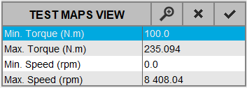
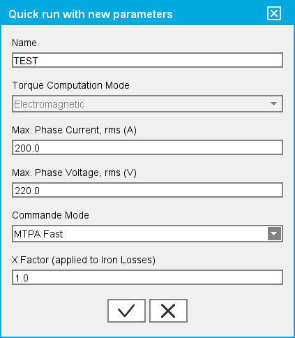
Quick run with new parameters
It's possible to create and run a new test with new values of some parameters. The possible parameters to modify are the parameters which no need a re-solving of the Flux project, but only a re-compute and re-display of maps.
The possible parameters to modify for a quick run are:
- Torque Computation Mode
- Max. Phase Current, rms (A)
- Max. Phase Voltage, rms (V)
- Command Mode (MTPA/MTPV)
- X Factor (applied to Iron Losses)
The maps will be updated in only few seconds.
- Open the Quick run with new parameters dialog box:Display the
wished test by double click on it.
→ the test are displayed on the center area in a new tab
→ The ribbon with Quick Run button appears
 Note: It's also possible to open the Quick run dialog box:
- by selecting the test in the list and by clicking on

- or by a right-click on the test and by selecting in the contextual menu → Quick run
→ the dialog is opened
- by selecting the test in the list and by clicking on
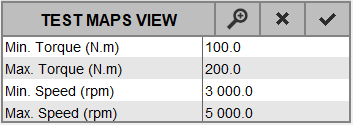
- Fill the fields with the new customs values and validate
→ a new test is automatically created in the TESTS table and the maps are generated in few seconds
Possible parameters to modify for a Quick Run
Torque computation mode
- For the torque computation, the Useful mode is only available with the TM and MS multi-positions computation modes (for which the iron losses are computed).
- With the MS mono-position computation mode, the iron losses are not computed, so the Useful mode is not available, the torque will therefore be computed with the Electromagnetic mode.
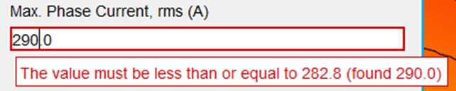
Max. Phase Current, rms (A)
- Imax is the initial value of the “Max. Phase Current, rms (A)”. It will always be the value of the original fully computed test, even if the test is post-processed from another post-processed test.
- Then ImaxNew should be 0.5*Imax ≤ IMaxNew ≤ Imax otherwise
extrapolation may cause accuracy loss. A warning message is displayed in
that case.

- ImaxNew < √2*Imax otherwise an error message will be
displayed
Command mode
- from MTPA to MTPV
- from MTPV to MTPA