Finite element computation, approximation functions

Introduction

This paragraph deals with the approximation functions in finite element computation in magnetic applications for the formulations automatically chosen (Magnetic scalar potential and electric vector potential):

order of the approximation functions: first order / second order
type of the approximation functions: edge/nodal

Order of elements and approximation functions

Flux provides to the user:

different types of finite elements mesh: 1^st order mesh or 2^nd order mesh
different types of approximation functions: linear functions (first order) or quadratic functions (second order)

The order of the approximation functions is connected by default with the mesh order, as presented in the table below.

Mesh	Position of nodes	Approximation function
1st order	Vertexes	Linear (polynomial of first order)
2nd order	Vertexes + middle of edges	Quadratic (polynomial of second order)

Flux dissociates the order of the approximation functions and the mesh order. Thus, the user can combine a 1st order mesh with approximation functions of the second order and the other way round*.

Note: * In the case when the user chooses approximation functions of the second order with a 1^st order mesh, the software automatically imposes a 2^nd order mesh (necessary for a computation with approximation functions of the second order).

Nodal or edge approximation function

Flux provides to the user:

the edge approximation functions (computation on the edges of finite element and storage of information in the middle node of edges)
the nodal approximation functions (computation on the nodes of the finite element)

The edge functions are provided only for the electric vector potential T. The approximation functions for the scalar magnetic potential Φ are of the nodal type.

Therefore, the use of the edge functions is applied to the regions of the solid conductor type (Transient Magnetic and Steady state AC Magnetic applications).

Caution

The edge formulations are compulsory (otherwise the results are false) under the following conditions:

solid conductors
presence of induced currents tangent to the device edges. These edges are the edges of the inside corners of the device.

These conditions are illustrated in the following figure.

Example: computation of the eddy currents in a solid conductor of the thin plate type in the presence of cracks.

Modifying the default choices

The user does not have to modify the order or the type of the approximation functions. The default choices are adapted to the most situations. However, these choices can be brought to a change under certain particular conditions.

This is why the two operation modes are described in the following sections:

automatic mode: default choice
manual mode: user’s choice

Automatic mode

In automatic mode, the order of the nodal approximation functions follows the order of the mesh:

if the mesh is of the 1^st order, the nodal approximation functions are of the first order
if the mesh is of the 2^nd order, the nodal approximation functions are of the second order

If there are regions of the solid conductor type (formulation in electric vector potential), the approximation functions are the edge functions that require a 2^nd order mesh. The generation of 2^nd order mesh is then automatically carried out.

The computation is therefore carried out under the following conditions:

Magnetic scalar potential: nodal approximation functions (2^nd order)
Electric vector potential: edge approximation functions

In manual mode

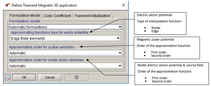
In manual mode, the user can modify the order (1^st order / 2^nd order) and the type of approximation functions (nodal type/edge type for the electric vector potential). These modifications are carried out in the dialog box of the application definition as presented in the figure below.

Advice

For a huge project, if the memory is not enough during solving process, it is possible to decrease the memory by choosing the vector variables approximation order of first order. It allows earning solving time and memory, despite a light results accuracy degradation.