Compose-3500: Linear Algebra Operations in OML
Tutorial Level: Beginner
The Compose OML language provides a linear algebra toolbox to solve linear system problems, analyze a matrix, and perform matrix decomposition, for example.
- Solve linear systems of equations.
- Perform basic matrix analysis.
- Perform matrix decomposition.
Solve Linear Systems of Equations
-
To solve systems of linear equations
Ax = bfor x, use\directly or the mldivide function, which returns the same result. The algorithm selected internally depends on the matrix A.If
Ais a square matrix, OML returns the unique solution:% solve linear equation A*x = b when A is square % unique result is returned A = [9 13 5 2; 1 11 7 6; 3 7 4 1; 6 0 7 10]; b = [-1 6 3 -4]'; x1 = mldivide(A,b) x2 = A\b disp('check if x1 equals x2') isequal(x1,x2)Results in Compose are shown below:

If
Ahas fewer equations than unknowns, the system is under determined, having fewer rows than columns, and the solution is not unique. The computed result is the least squares solution with the minimum norm:% solve under determined equation A*x = b % there are fewer equations than unknowns in this case % computed result is the least squares solution with the minimum norm A = [1 1 1; 1 1 2]; b = [1 3]'; x1 = mldivide(A,b) x2 = A\b disp('check if x1 equals x2') isequal(x1,x2)Results in Compose are shown below:

If
Ahas more equations than unknowns, the system is over determined, having more rows than columns, and there is no solution. The computed result is the unique least squares solution:% solve over determined equation A*x = b % A is rectangular and has more rows than columns % the unique least squares solution is computed in this case A = [2 1; -3 1; -1 1]; b = [-1 -2 1]'; x1 = mldivide(A,b) x2 = A\b disp('check if x1 equals x2') isequal(x1,x2)Results in Compose are shown below:

If
Ais singular matrix, a warning is raised:% solve linear equation A*x = b when A is singular % it will raise a warning in this case A = [16 2 3 13; 5 11 10 8; 9 7 6 12; 4 14 15 1]; b = [1 1 1 1]'; x1 = mldivide(A,b) x2 = A\b disp('check if x1 equals x2') isequal(x1,x2)Results in Compose are shown below:

-
To solve
Ax = b, if you have a priori knowledge about matrixA(lower triangular, positive definite, general rectangular, and so on), you could choose the linsolve function to enhance the efficiency of the calculation. Basically, linsolve works exactly as\, but it has an extra input argument to specify the characteristic of matrixA. -
Ax = bis solved, but you may want to solvexA = b. In this case,/or the mrdivide function can be used with same logic as in previous section.
Basic Matrix Analysis
This section introduces two matrix analysis cases, one with matrix inversion, and another with Eigenvalues and Eigenvectors.
-
Calculate inverse of a matrix.
When a matrix is square and non-singular, the inverse is computed with the inv function:
% calculate non-singular matrix inversion
format(3,2);
M = [1 2 -3;4 5 6;-7 8 0]
Inv_M = inv(M)
M2 = inv(inv(M))
find((M - M2) > 10*eps)
Results in Compose are shown below:

Observe above that inv(inv(M)) is equal to M, within round off error. But when M is not a square or is a singular matrix, inv returns an error or a warning. Alternatively, you can calculate its Moore-Penrose inverse, or pseudoinverse. If A2 is the pseudoinverse matrix of A1, it should satisfy the following:
A2*A1*A2 = A2
A1*A2*A1 = A1
conj(A1*A2) = A1*A2
conj(A2*A1) = A2*A1
Verify if it obeys all four rules in OML:
% calculate singular matrix inversion using pinv
format(3,2)
A1 = [1 2 3;4 5 6;7 8 9];
disp('A2 vs. A2*A1*A2')
A2 = pinv(A1)
A2*A1*A2
disp('A1 vs. A1*A2*A1')
A1
A1*A2*A1
isequal(conj(A1*A2),A1*A2)
isequal(conj(A2*A1),A2*A1)
Results in Compose are shown below:

-
Calculate Eigenvalues and Eigenvectors of a matrix.
An Eigenvalue of a square matrix is a vector,
, that does not change direction under a linear transformation with the matrix, which can be described with the following equation:
where
is a scalar known as the eigenvalue associated with the eigenvector
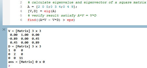
. In OML, use the eig function to compute this.
% calculate eigenvalue and eigenvector of a square matrix
A = [2 0 0;0 3 4;0 4 9];
[V,D] = eig(A)
% verify result satisfy A*V = V*D
find((A*V - V*D) > eps)
Results in Compose are shown below:

Matrix Decomposition
A matrix decomposition is a factorization of a matrix into a product of matrices. There are many different matrix decompositions; each finds use among a particular class of problems. This section introduces the LU and QR decomposition.
-
LU decomposition.
LU decomposition factors a matrix as the product of a lower triangular matrix and an upper triangular matrix. In OML, the lu function is used:
% LU decomposition
A = [4 3 1;0 6 3;1 2 4]
[L,U] = lu(A)
% verify if
L*U = A
Results in Compose are shown below:

Observe that
LandUreturned by this function are lower and upper triangular matrices, andL*Uis equal to the original matrixA. -
QR decomposition.
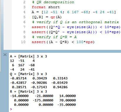
QR decomposition factors a matrix as the product of an orthogonal matrix Q and an upper triangular matrix R. In OML, the qr function is used:
% QR decomposition
format short
A = [12 -51 4; 6 167 -68; -4 24 -41]
[Q,R] = qr(A)
% verify if Q is an orthogonal matrix
assert((Q'*Q - eye(size(A))) < 10*eps)
assert((Q*Q' - eye(size(A))) < 10*eps)
% verify if Q*R = A
assert((A - Q*R) < 100*eps)
Results in Compose are shown below:

Observe that
Qis an orthogonal matrix,Ris an upper triangular matrix, andQ*Ris equal toA, within round off error. - For all complete scripts, please refer to install_dir/tutorials/.
