Inputs
1. Introduction
The total number of user inputs is equal to 15.
Among these inputs, 10 are standard inputs and 5 are advanced inputs.
2. Standard inputs
2.1 Current definition mode
There are 2 common ways to define the electrical current.
Electrical current can be defined by the current density in electric conductors.
In this case, the current definition mode should be « Density ».
Electrical current can be defined directly by indicating the value of the line current (the peak value is required).
In this case, the current definition mode should be « Current ».
2.2 Current density, peak
When the choice of current definition mode is “ Density ”, the peak value of the current density in electric conductors “ Current density, peak” ( Current density in conductors, peak value ) must be provided.
So, there can be a difference (sometimes very important) between the targeted value and the current density in conductors resulting from computations. In any case, the resulting value of current density in conductors is computed and displayed in the table of results.
2.3 Line current, peak
When the choice of current definition mode is “ Current ”, the peak value of the line current supplied to the machine: “ Line current, peak” ( Line current, peak value ) must be provided.
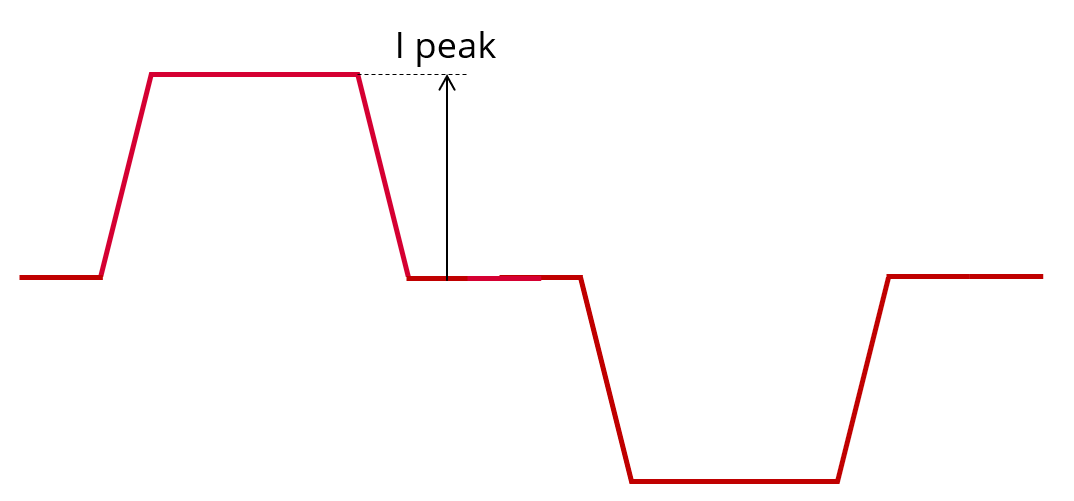 |
| Definition of the line current – Peak value |
2.4 Speed
The imposed “ Speed ” ( Speed ) of the machine must be set.
2.5 Control angle
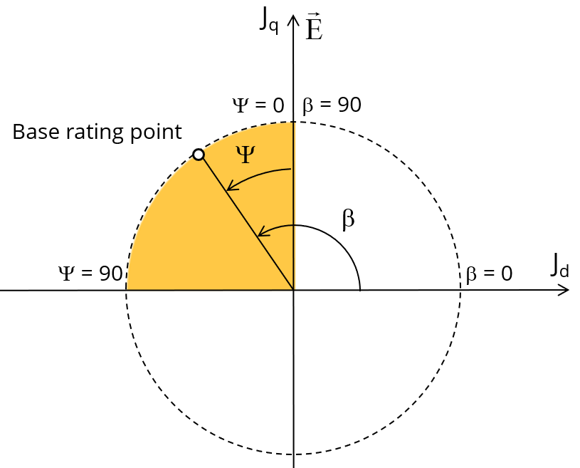
Considering the vector diagram shown below, the “ Control angle ” is the angle between the electromotive force E and the electrical phase current (J) (Ψ = (E, J)).
The default value is 0 degrees. It is an electrical angle. It must be set in a range of -90 to 90 degrees.
 |
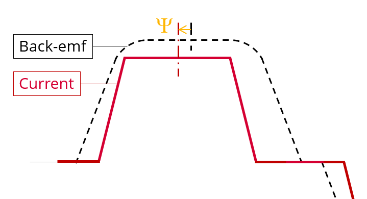 |
| Definition of the control angle Ψ | |
2.6 Conduction angle
The “ Conduction angle ” ( Electrical conduction angle ) is the time during which phase is powered with current.
The default value is 120 degrees (typical 6 steps control mode with a 6-transistor power electronics converter). It is an electrical angle. It must be set in a range of 0 to 180 degrees.
For more details refer to the following illustration “Conduction angle” and Rise and fall angle”.
2.7 Rise and fall angle
The “ Rise and fall angle ” ( Rise and fall angle of the current in electrical angle ) represents the time constant needed for current rise from 0 to the peak value of the current or current fall from the peak value to 0.
The default value is 6 degrees. It is an electrical angle. It must be set in a range of 0 to 90 degrees.
To be noted that the “Rise and fall angle” must be compatible with the “Conduction angle”. For instance, the “Rise and fall angle” must be strictly lower than half the value of “Conduction angle”. In any case, the addition of “Rise and fall angle” and the “Conduction angle” must be lower than 180 degrees.
For more details refer to the following illustration “Conduction angle” and Rise and fall angle”.
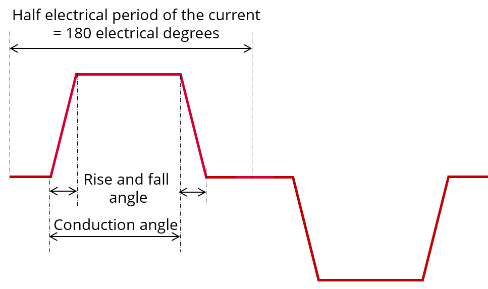 |
| Conduction angle” and “Rise and fall angle” |
2.8 Iron loss computation
The “ Iron loss computation ” ( Iron loss computation: Yes / No ) allows to compute or not to compute the value of the iron losses in the magnetic circuit and display the corresponding losses versus time over an electric period.
The default value is “No”.
The iron losses will be computed on both stator and rotor parts.
- Iron losses are obtained through post-processing of finite elements analysis results (and not directly through the transient simulation), so to have a consistent power balance the useful torque is deduced from those losses.
- This choice influences the computation time. So, the user can choose first computing the working point without iron loss results
2.9 Losses in magnets computation
The “ Losses in magnets computation “( Losses in magnets computation: Yes / No ) allows to compute or not to compute the value of Joule losses in magnets and display them versus time over an electric period.
The default value is “No”.
If the user chooses to compute the losses in magnets, they are directly computed during the transient finite element simulation. It means that the obtained electromagnetic torque already takes them into account.
2.10 Additional losses
The “ Additional losses ” ( Additional loss percentage of electric losses ) must be provided.
It is used to consider losses which are not computed (like losses due to eddy currents, proximity effects due to electronic devices). Thus, these additional losses will be considered for computing the power balance and efficiency.
Additional losses must be evaluated as a percentage of total losses (Joule losses in coils and magnets and iron losses occurring in stator and rotor).
The default value is 0. This input parameter value must be set in a range of 0% to 100% when the unit is % and 0 to 1 when represented in “P.U.” (“Per Unit”).
When the default value is equal to 0, it means the power balance is computed without considering additional losses.
3. Advanced inputs
3.1 Minimum number of computations per electrical period
The user input “ Min. no. comp. / elec. period ” ( Minimum number of computations per electrical period ) influences the accuracy of results and the computation time. It allows giving a floor value for the number of computation per electrical period.
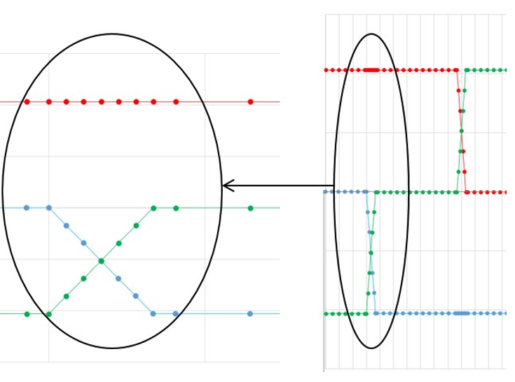
Note: In any cases, the real number of computations per electrical period will be higher because the number of computations within the rise and fall period is adjusted through an internal process. The distribution of computation points is illustrated below: Definition of the number of computations per electrical period.
The default value is equal to 87. The default value provides a good compromise between the accuracy of results and computation time. The minimum allowed value is 87.
 |
| Definition of the number of computations per electrical period |
3.2 Rotor initial position mode
The computation of the test « Working point / Square wave / Motor » is performed by considering a relative angular position between rotor and stator.
This relative angular position corresponds to the angular distance between the direct axis of the rotor north pole and the axis of the stator phase 1 (reference phase).
According to the input “ Rotor initial position mode ”, the angular position can be defined either automatically using an internal computation process « Auto » (Automatic) or specified by the user « User » (User).
By default, the “ Rotor initial position mode ” is set to “ Auto ”.
3.3 Rotor initial position
When the “ Rotor initial position mode ” is set to “ Auto ”, the initial position of the rotor is automatically defined by an internal computation process .
The resulting relative angular position corresponds to the alignment between the axis of the stator phase 1 (reference phase) and the direct axis of the rotor north pole.
When the “ Rotor initial position mode ” is set to “ User ”, the initial position of the rotor considered for computation must be set by the user in the field « Rotor initial position » (Rotor initial position). The default value is equal to 0. The range of possible values is [-360, 360].
For more details, please refer to the section "Rotor and stator phase relative position".
3.4 Skew model – Number of layers
When the rotor magnets or the stator slots are skewed, the number of layers used in Flux Skew environment to model the machine can be modified: “ Skew model - No. of layers” ( Number of layers for modelling the skewing in Flux Skew environment ).
3.5 Mesh order
To get the results, the original computation is performed using a Finite Element Modeling (inside Flux software).
Two levels of meshing can be considered for this finite element calculation: first order and second order.
This parameter influences the accuracy of results and the computation time.
By default, second order mesh is used.
3.6 Airgap mesh coefficient
The advanced user input “ Airgap mesh coefficient ” is a coefficient which adjusts the size of mesh elements inside the airgap. When the value of “ Airgap mesh coefficient ” decreases, the mesh elements get smaller, leading to a higher mesh density inside the airgap and increasing the computation accuracy.
The imposed Mesh Point (size of mesh elements touching points of the geometry), inside the Flux software, is described as:
MeshPoint = (airgap) x (airgap mesh coefficient)
Airgap mesh coefficient is set to 1.5 by default.
The variation range of values for this parameter is [0.05; 2].
0.05 giving a very high mesh density and 2 giving a very coarse mesh density.
However, this always leads to a huge number of nodes in the corresponding finite element model. So, it means a need of huge numerical memory and increases the computation time considerably.