Inputs
1. Introduction
The total number of user inputs is equal to 11.
Among these inputs, 5 are standard inputs and 6 are advanced inputs.
2. Standard inputs
2.1 Mechanical torque
The value of the targeted “ mechanical torque” must be provided.
2.2 Speed
The value of the targeted “ Speed” ( Targeted speed ) must be provided.
2.3 Command mode
Two commands are available: Maximum Torque Per Voltage (MTPV) and Maximum Torque Per Amps (MTPA) command mode.
For the base speed point computation, both commands lead to the same results. In fact, the base speed point corresponds to the working point which maximize the mechanical torque at maximum current and at maximum voltage.
Following this, MTPA and MTPV commands give the same results on this test.
2.4 Ripple torque analysis
The “ Ripple torque analysis ” (Additional analysis on ripple torque period: Yes / No) allows to compute or not to compute the value of the ripple torque and to display the corresponding torque versus the angular position over the corresponding ripple torque period.
The default value is “No”.
- This choice influences the accuracy of results and the computation time. The peak-peak ripple torque is calculated. This additional computation needs addition computation time.
- In case of “ Yes ”, the ripple torque is computed. Then, the flux density in regions and the magnet demagnetization rate are evaluated through the ripple torque computation.
- In case of “ No ”, the ripple torque is not computed. Then, the flux density in regions and the magnet demagnetization rate are evaluated by considering the Park’s model computation.
2.5 Additional losses
The “ Additional losses ” ( Additional loss percentage of electric losses ) must be provided.
It is used to consider losses which are not computed (like losses due to eddy currents, proximity effects due to electronic devices). Thus, these additional losses will be considered for computing the power balance and efficiency.
Additional losses must be evaluated as a percentage of total electrical losses (Joule + iron).
The default value is 0. This input parameter value must be set in a range of 0% to 100% when the unit is in % and 0 to 1 when represented in “P.U.” (“Per Unit”).
When the default value is equal to 0, it means the power balance is computed without considering additional losses.
3. Advanced inputs
3.1 Number of computations for J d , J q
First, it is needed to compute the D-axis and Q-axis flux linkage in the J d - J q plane.
The process to find the working point uses a current map in J d - J q plane where a grid is defined.
The number of computation points along the d-axis and q-axis can be defined with the user input «No. comp. for current J d , J q » ( Number of computations for D-axis and Q-axis currents ).
The default value is equal to 5. This default value provides a good compromise between accuracy and computation time. The minimum allowed value is 5.
3.2 Number of computations per ripple torque period
The number of computations per ripple torque period is considered when the user has chosen to perform a “Ripple torque analysis” (i.e. answered “Yes” to the standard input “Ripple torque analysis”).
The user input “ No. comp. / ripple period ” (Number of computations per ripple torque period) influences the accuracy of results (computation of the peak-peak ripple torque) and the computation time.
The default value is equal to 30. The minimum allowed value is 25. The default value provides a good compromise between the accuracy of results and computation time.
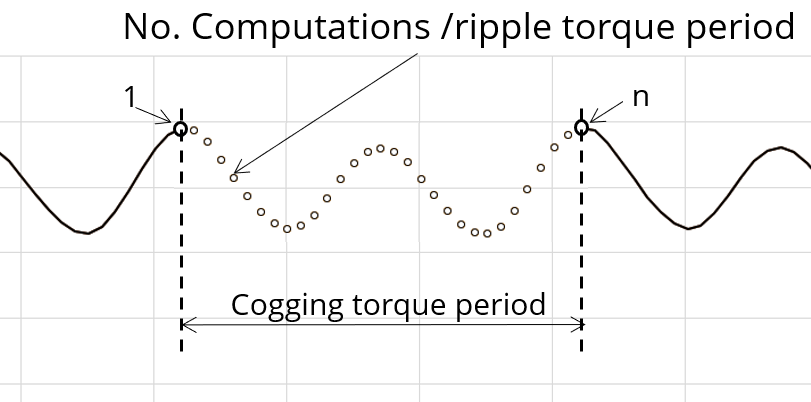 |
| Definition of the number of computations per ripple torque period |
3.3 Rotor initial position mode
The computation is performed by considering a relative angular position between rotor and stator.
This relative angular position corresponds to the angular distance between the direct axis of the rotor north pole and the axis of the stator phase 1 (reference phase).
According to the input “ Rotor initial position mode ”, the angular position can be defined either automatically using an internal computation process « Auto » (Automatic) or specified by the user « User » (User).
By default, the “ Rotor initial position mode ” is set to “ Auto ”.
3.4 Rotor initial position
When the “ Rotor initial position mode ” is set to “ Auto ”, the initial position of the rotor is automatically defined by an internal computation process.
The resulting relative angular position corresponds to the alignment between the axis of the stator phase 1 (reference phase) and the direct axis of the rotor north pole.
When the “ Rotor initial position mode ” is set to “ User ”, the initial position of the rotor considered for computation must be set by the user in the field « Rotor initial position mode » The default value is equal to 0. The range of possible values is [-360, 360].
For more details, please refer to the section dedicated to the rotor and stator phase relative position.
3.5 Skew model – Number of layers
When the rotor magnets or the stator slots are skewed, the number of layers used in Flux Skew environment to model the machine can be modified: “ Skew model - No. of layers” ( Number of layers for modelling the skewing in Flux Skew environment ).
3.6 Mesh order
To get the results, the original computation is performed using a Finite Element Modeling (inside Flux software).
Two levels of meshing can be considered for this finite element calculation: first order and second order.
This parameter influences the accuracy of results and the computation time.
By default, second order mesh is used.
3.7 Airgap mesh coefficient
The advanced user input “ Airgap mesh coefficient ” is a coefficient which adjusts the size of mesh elements inside the airgap. When the value of “ Airgap mesh coefficient ” decreases, the mesh elements get smaller, leading to a higher mesh density inside the airgap, increasing the computation accuracy.
The imposed Mesh Point (size of mesh elements touching points of the geometry), inside the Flux software, is described as:
MeshPoint = (airgap) x (airgap mesh coefficient)
Airgap mesh coefficient is set to 1.5 by default.
The variation range of values for this parameter is [0.05; 2].
0.05 giving a very high mesh density and 2 giving a very coarse mesh density.
However, this always leads to a huge number of nodes in the corresponding finite element model. So, it means, a need of huge numerical memory and increases the computation time considerably.