Define Iron Loss parameters

1. Iron losses model - Main principles

The mathematical formula used in the material database to compute the iron losses is:

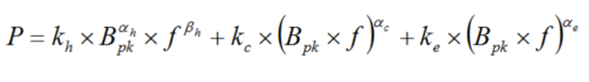Note: Iron loss model is only used for lamination.


Label	Definition
k _h	Hysteresis loss coefficient
α _h	Exponent of B for the hysteresis losses
β _h	Exponent of f for the hysteresis losses
k _c x kα _c	Classical loss coefficient – Sine wave
k _c	Classical loss coefficient – Any wave Automatically computed from the sine wave value – The field is grayed out.
α _c	Exponent of B and f for the classical losses
K _e x kα _e	Excess loss coefficient – Sine wave
k _e	Excess loss coefficient – Any wave Automatically computed from the sine wave value – The field is grayed out.
α _e	Exponent of B and f for the excess losses

Note: The formula above is not homogeneous with considered the units.

Indeed, it represents a correspondence between the flux density associated with the frequency and the resulting iron loss amount.

The coefficients listed above are completely independent of units.

P represents the amount of iron losses per cubic meter. This quantity is computed by considering B in Tesla and f in Hertz. The coefficients are always defined by considering these reference units.

The user can use other units for defining the iron losses or flux density for example.The corresponding quantities are transformed to come back to original units (Tesla, Hz and W/m3).

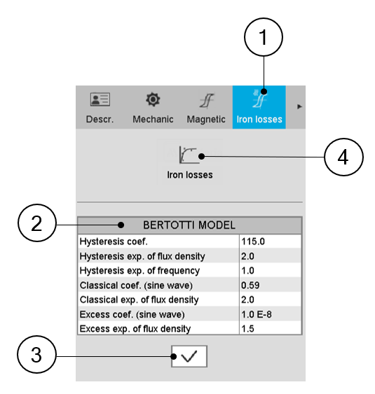
When creating a new material or when editing the properties of an existing one, a tab is dedicated to the magnetic data. In this tab, iron loss coefficients must be given.



Definition of iron loss coefficients
1	Category dedicated to iron losses.
2	Parameters defining the iron losses according to the model described above (Bertotti model).
3	Click “ok” button to validate the inputs
4	Click in the fitting icon in order to get an iron losses model from measured data.

2. How to define iron loss parameters

2.1 Overview

Three main methods are provided to help the users find the relevant values to consider for the iron loss parameters. The choice of the method depends on the data that the user has for the lamination to consider.

Three cases are considered:

One measurement point is characterized: Amount of iron losses corresponding to the values (frequency, induction).
Two measurement points are characterized: Amount of iron losses corresponding to the values (frequency, induction).
Several curves of iron losses in function of flux density for different values of frequency which corresponds to a map of Iron losses in f - B plane (where f= frequency and B=flux density).

2.2 Case 1: From one measurement point



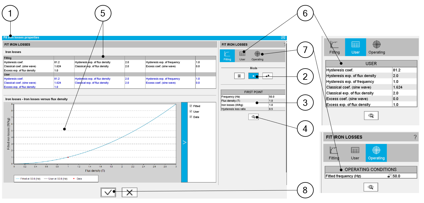Definition of iron loss coefficients – from one measurement point
1	Dialog box dedicated to fit the iron loss parameters. Located in the “iron losses” category when visualizing or editing the material properties.
2	Choice of the method to find iron loss parameters (1 point in this example).
3	Measurement characteristics: Frequency, Induction (magnetic flux density B), Iron losses (amount of iron losses) Hysteresis loss ratio. Note: Hysteresis loss ratio is the ratio between the hysteresis losses and the total amount of iron losses.
4	When input parameters characterizing the measurement point are defined, click the button Fit to run the optimization process. This process computes the set of iron loss parameters that allow targeting the considered measurement point.
5	The iron loss input parameters are deduced and displayed in the result table and the corresponding curve, Losses versus B (magnetic flux density) are displayed.
6	The user can adjust one or all the parameters of the iron losses model. To do so user tab must be selected by clicking on its icon. The resulting modification is directly displayed in the output area.
7	It is possible to select a frequency to visualize the behavior of the resulting iron loss curve. To do so, use the “Operating” tab. Note: If the chosen frequency is not one of those used for the fitting (from the user inputs), the measurement points (in red) will not be displayed.
8	Validation of iron loss parameters is achieved by clicking on this button. Moreover, it is also possible to cancel the computation of iron loss parameters.

2.3 Case 2: From two measurement points



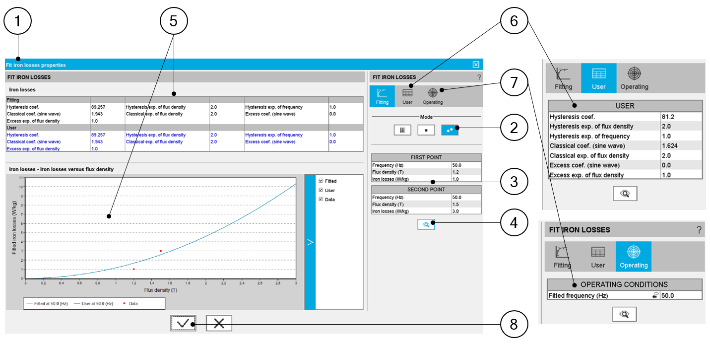Definition of iron loss coefficients – from two measurement points
1	Dialog box dedicated to fit the iron loss parameters. Located in the “iron losses” category when visualizing or editing the material properties.
2	Choice of the method to find iron loss parameters (2 points in this example).
3	Measurement characteristics to give for each measurement point: Frequency (It is highly recommended to take 2 different frequencies as boundaries of the working area) Induction (magnetic flux density B) Iron losses (amount of iron losses)
4	When input parameters characterizing the two measurement points are defined, click on the Fit button to run the optimization process. This process computes the set of iron loss parameters that allow targeting the considered measurement points.
5	The resulting iron loss input parameters are deduced and displayed in the result table and the corresponding curve; Losses versus B (magnetic flux density) is displayed.
6	The user can adjust one or all the parameters of the iron losses model. To do so user tab must be selected by clicking on its icon. The resulting modification is directly in the outputs area.
7	It is possible to select a frequency to visualize the behavior of the resulting iron loss curve. To do so, use the “Operating” tab. Note: If the chosen frequency is not one of those used for the fitting (from the user inputs), the measurement points (in red) will not be displayed.
8	Validation of iron loss parameters is achieved by clicking on this button. Moreover, it is also possible to cancel the computation of iron loss parameters.

Warning: When characterizing the iron loss parameters by using the method with two measurement points there are two things to be known:

Firstly, the internal process uses a genetic algorithm to compute the iron loss parameters.

When the same frequency is considered for the two targeted points, this can lead to a disparity on the resulting iron loss parameters. It means that, the same set of inputs provide sets of iron loss parameters, which can be different. However, the resulting iron loss model gives the same total amount of iron losses.
Note: The best way to use the method with two measurement points, is to consider two different frequencies. Thus, there is only one resulting set of iron loss parameters.

It is highly recommended to take 2 different frequencies as boundaries of the working area.

Moreover, check that the classical losses coefficient is positive before using the resulting iron loss model. If this coefficient is negative, please check the relevance of the original data.
Secondly, defining the iron loss parameters, with frequency different from the one which is considered for the computation of a working point in Motor Factory, can lead to wrong results.

The most accurate way to compute iron loss parameters is to use a map of iron losses in f - B plane (f= frequency and B=flux density) where iron losses are defined in function of flux density for different values of frequency.
Note: To be accurate the frequency and the flux density of the working point to be computed must be respectively in the range of frequencies and flux densities used to identify the iron loss parameters.

2.4 Case 3: From a map (file input)

Restriction:

The fitting function for defining the iron loss parameters from a map (Excel file inside in which several iron loss curves as a function of the flux density are available for different values of frequency) doesn’t work anymore.

This function worked in the previous version FluxMotor 2023.1.

One workaround consists in using the “Flux Material Identification” tool in Altair^®Flux^® for defining the parameters.

(ref.: FXM-16789).



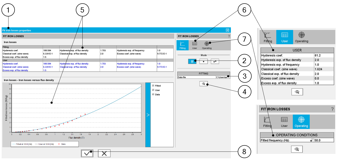Definition of iron loss coefficients – from a map
1	Dialog box dedicated to fit the iron loss parameters. Located in the “iron losses” category when visualizing or editing the material properties.
2	Choice of the method to find iron loss parameters (form input file in this example).
3	Select the Excel file inside of which several curves of iron losses with flux density functions are available for different values of frequency are defined. An example of file is shown below.
4	When the Excel file is selected, click on the Fit button to run the optimization process. This process computes the set of iron loss parameters targeting the considered measurement points.
5	The resulting iron loss input parameters are deduced and displayed in the result table and the corresponding curve; Losses versus B (magnetic flux density) is displayed.
6	The user can adjust one or all the parameters of the iron losses model. To do so user tab must be selected by clicking on its icon. The resulting modification is directly in the outputs area.
7	It is possible to select a frequency to visualize the behavior of the resulting iron loss curve. To do so, use the “Operating” tab. Note: If the chosen frequency is not one of those used for the fitting (from the user inputs), the measurement points (in red) will not be displayed.
8	Validation of iron loss parameters is achieved by clicking on this button. Moreover, it is also possible to cancel the computation of iron loss parameters.

Example of an Excel file to define the curves of iron losses in function of flux density for different values of frequency.

This corresponds to a map of Iron losses in f - B plane (where f= frequency and B=flux density).



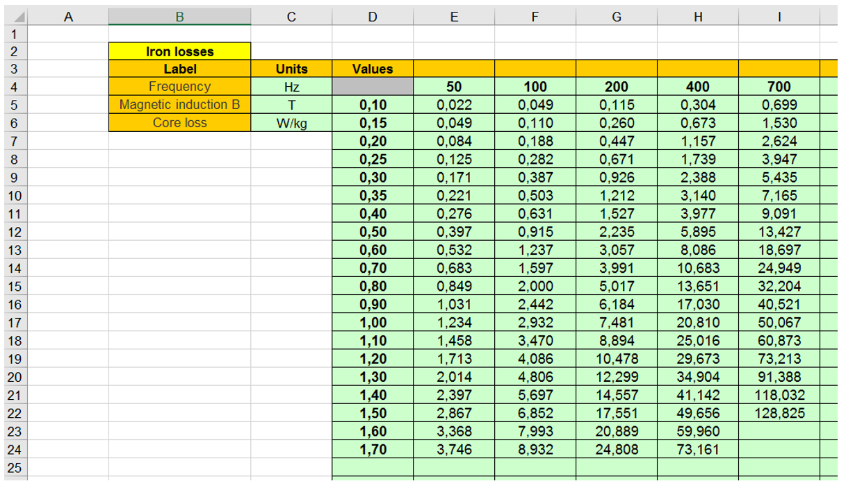Example of an Excel file to define iron loss parameters from a map

Note: The columns with the larger number of rows must be written first. At least three columns with the same number of rows must be written. In the example above, there are four columns with twenty rows.

Note: The exponent of B for the excess losses is set to 1.5 in the optimization process.