Create B(H) curve
1. Create a B(H) curve – Main principles
The model consists of a combination of a straight line and a curve. A coefficient allows for the adjustment of the knee shape for better approximation of the experimental curve.
The corresponding mathematical formula is written as follows:
 |
| μ0 | Permeability of vacuum. |
| μr | Initial relative permeability of the material. |
| H | Magnetic field (A/m). |
| Js | Magnetic polarization at saturation (T). |
| a |
Knee coefficient of the curve (a > 0 and a ≠ 1). The smaller coefficient will give, the sharper knee point. |
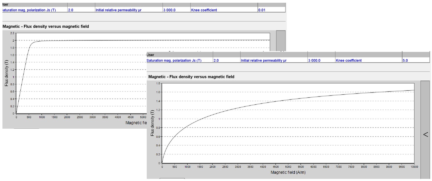
The impact of the knee coefficient “a” on the shape of the B(H) curve is illustrated in the below figure.
 |
|
Shape of B(H) curve with the function of knee coefficient. Left knee coefficient = 0.01. Right knee coefficient = 5 |
2. Create a B(H) curve – Process
A linear or a non-linear B(H) curve is considered.
In the first case, only the constant value of the relative permeability must be given by the user.
If a lamination is considered, the relative permeability of the lamination stack is automatically deduced.
If a non-linear B(H) curve is considered, these three main parameters of the magnetic characteristics must be defined:
-
The magnetic polarization at saturation J S
-
The magnetic permeability (µ r )
-
And the knee coefficient a
3. Define a B(H) curve from user input parameters
Here is the process to define the B(H) curve from the “Materials” application. In this example, it is considered that the user knows exactly the coefficients to be set.
 |
|
| Characterization of the B(H) curve | |
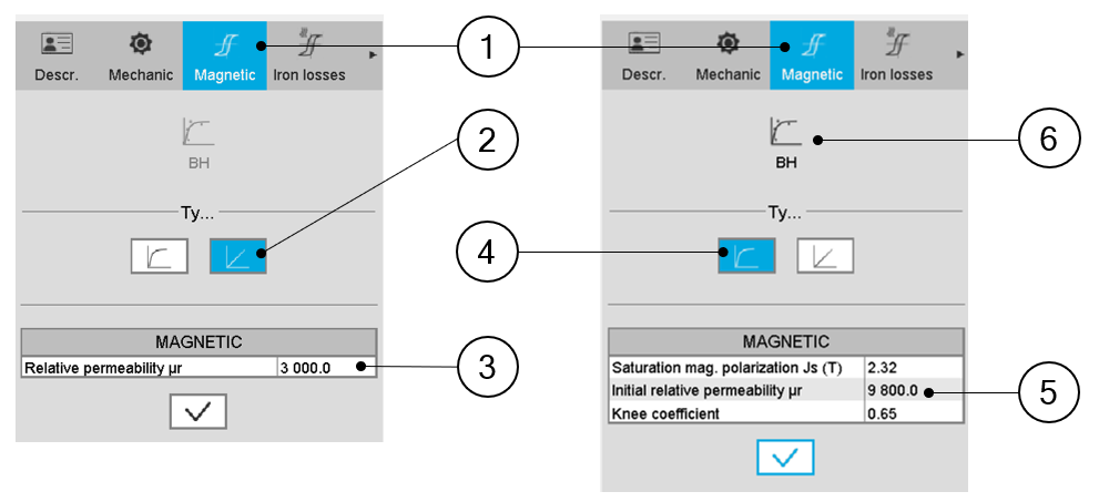
| 1 | When editing the properties of an existing material (lamination and solid families), a category is dedicated to the magnetic data. Hence, clicking on the “Magnetic” one can define the B(H) curve. |
| 2 | In the example above, the linear B(H) characteristic of a lamination is considered |
| 3 |
Only the relative permeability of the corresponding solid material is given. The resulting relative permeability of the lamination stack is automatically deduced (considering the stacking factor mentioned in the mechanical data). |
| 4-5 | In another example, the non-linear B(H) characteristic of a lamination is considered. |
| 6 | The three main parameters of the magnetic characteristic that must be
given are:
|
| 7 | Another method is possible to define the B(H) curve characteristics of a
material.If the user has measurement or computation points representing the
B(H) curve to model, it is possible to import these data to define the
corresponding characteristics.This consists of importing a B(H) curve via an
Excel file and identifying the three parameters J S , µ
r and knee coefficient with an optimization process. Click on the icon “Fit” to run this process. |
4. Define a B(H) curve from experimental data
Here is the process to define the characteristics of the B(H) curve from the importation of a series of points representing the B(H) curve listed in an Excel file.
 |
|
| Identification of the B(H) curve characteristics | |
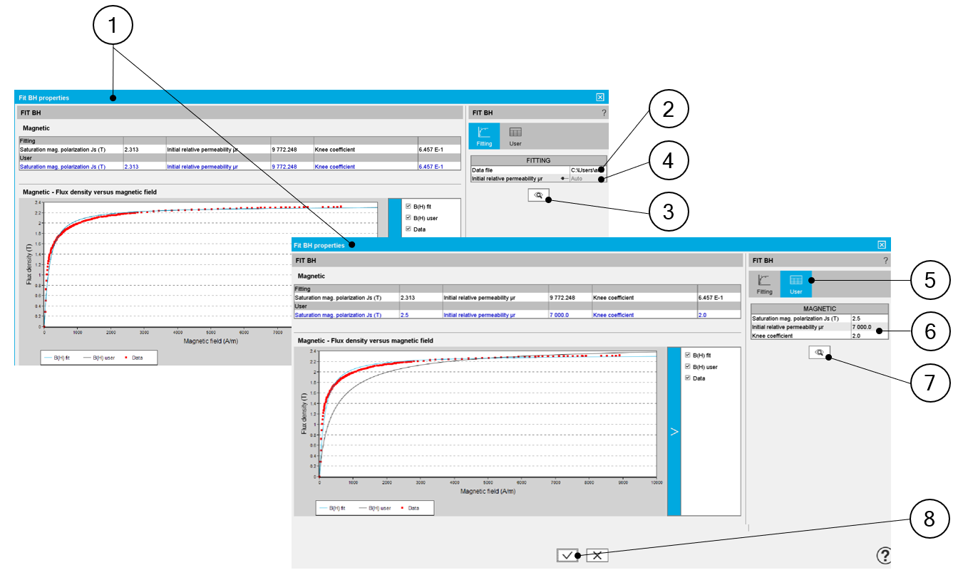
| 1 | Dialog box allowing the characterization of the B(H) curve imported from an Excel file |
| 2 | Path where Excel file to be imported is stored. See an example of Excel file below. |
| 3 | Accept the import of the Excel file data. hen importing an Excel file, points representing the B(H) curve are listed. An optimization process automatically computes and displays the corresponding characteristics Js, µr and a. At the same time three curves are displayed: Red points are the imported points (listed in the Excel file) Blue curve is the resulting curve computed by the optimization process. This corresponds to the computed characteristics and displayed just after the computation. The black curve shows modifications induced if the characteristics Js, µr and a are changed by the user. |
| 4 | In this field, two choices are available:
|
| 5 |
The user can adjust one or all the three main characteristics of the B(H) curve: Js, µr and a. To do so user tab must be selected by clicking on its icon. The resulting modification is directly displayed on the graph below. |
| 6 | Adjust the three variables to get a new user curve. |
| 7 | Accept the user values modification by clicking this button. |
| 8 |
The last values of JS, µr and a, written in the “user” input fields are validated when the user clicks on this button. It is possible to cancel the creation of the B(H) curve model. In this case, the previous values defined before opening this dialog box are reset. |
Example of an Excel file to define the B-H curves parameters.
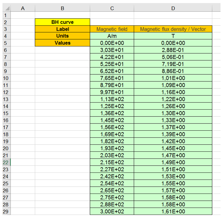 |
| Example of an Excel file to define the B(H) curve parameters |