Home
ProMan
The ProMan component includes wave propagation models for different scenarios and network planning simulators for various air interfaces.
Results
Evaluation of Results
Probability Density Function (PDF)

Welcome
Release Notes
See what's new in the latest release.
Get Started
The WinProp Getting Started Guide contains step-by-step instructions on how to get started with WinProp.
Examples
The Altair installation directory contains a collection of examples that shows you WinProp concepts and essentials.
Introduction to WinProp
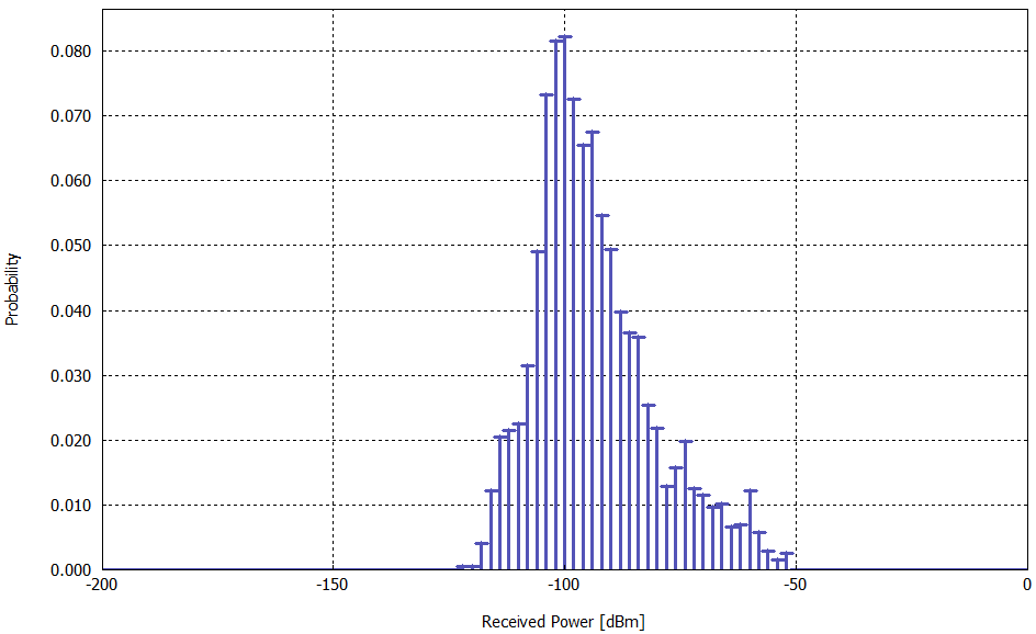
WinProp is a complete suite of tools in the domain of wireless propagation and radio network planning. With applications ranging from satellite to terrestrial, from rural via urban to indoor radio links, WinProp’s innovative wave propagation models combine accuracy with short computation time.
Typical Workflow in WinProp
View the typical workflows when working with propagation simulations in specific scenarios, how to add a network planning to a propagation simulation, include a receiver pattern, set up a time-variant scenario, include multiple-input multiple-output (MIMO) at both the base station and the mobile station, connectivity analysis of sensor networks and optimization.
WallMan
The WallMan component offers a convenient facility to generate and edit vector building databases.
TuMan
The TuMan tool enables you to generate and modify tunnel scenarios.
AMan
Use AMan to generate, edit and analyze a single antenna. Superimpose multiple antennas radiating similar signals to determine the actual antenna pattern while taking into consideration the local environment.
ProMan
The ProMan component includes wave propagation models for different scenarios and network planning simulators for various air interfaces.
- Introduction to Propagation Manager (ProMan)
  Predict path loss between transmitter and receiver with ProMan. Perform network planning including the wireless standards (the air interfaces) and including multiple transmitters/receivers (multiple base stations).
- Propagation Projects
- Network and Base Station Planning Projects
- MIMO Analysis Through Post-Processing
- Results
  - Display of Results
  - Modification of Results
  - Evaluation of Results
    - Information
    - Probability Density Function (PDF)
    - Cumulated Probability Density Function (CDF)
    - Comparison to Measurements
      Prediction results can be compared with measurement data in ProMan.
    - Reports of Monte Carlo Simulation
      The traffic simulation report in ProMan based on the Monte Carlo approach that evaluates the numbers of served, blocked and not assigned mobiles (users) for each application and for each cell.
  - Analysis of the Radio Channel
    Additional channel characteristics like channel impulse responses, spatial channel impulse responses and angular profiles can be displayed for user-defined locations in separate graphs.
  - Measurements
    The most important criterion to measure the performance of a prediction model is the accuracy. The accuracy of a prediction models can be analyzed by comparing simulation results with measurements.
  - Types of Results
    View the available result types and the corresponding file extensions.
- Addenda
- Parallel Processing
  Use parallel MPI processes to solve a problem efficiently using the standard ray tracing model (SRT).
- Default Shortcut Keys
  View the default shortcut keys available for ProMan for faster and easier operation.
Methods
WinProp includes empirical and semi-empirical models (calibration with measurements possible), rigorous 3D ray-tracing models as well as the unique dominant path model (DPM).
Main Applications
In WinProp various air interfaces and applications are pre-defined: broadcasting, cellular, wireless access, WiFi, sensor networks, ICNIRP and EM compliance.
WinProp Utilities
The WinProp utilities consist of the Launcher utility and the Updater.
Appendix
Reference information is provided in the appendix.

Probability Density Function (PDF)

ProMan offers the possibility to determine the probability density function for each type of simulation result, click Analysis > Display PDF (Probab. Density Fct) of Values, where you can select whether the PDF is determined for one of the following:

all prediction planes and all horizontal layers
all horizontal prediction planes
prediction planes and surfaces only
currently active horizontal prediction plane
zoomed area of the currently active horizontal plane

After selecting the area to be evaluated, you have to specify the quantization interval, which is used to discretize the result data.

Note: Unpredicted result pixels (result values which are set to not computed) are not considered for the generation of the PDF.

Figure 1. Example of a probability density function of a received power prediction.