
Tutorial: Conjugate Heat Transfer
Tutorial Level: Intermediate Learn how to run a conjugate heat transfer analysis with a simple model.
Import Geometry
- From the menu bar, select .
-
Browse to your working directory, select CHT_Tutorial.x_b,
and click Open.
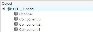
The model opens in the modeling window.
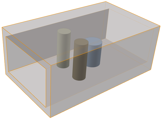
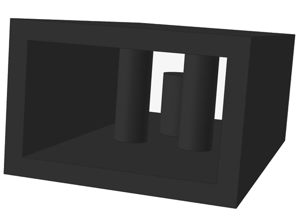
The model is comprised of the following parts:- Channel
- Component 1
- Component 2
- Component 3You can view these parts in the Object Browser:
Designate the Bounding Solid Domain
-
Click the Bounding Solid icon.
 Tip: To find and open a tool, press Ctrl+F. For more information, see Find and Search for Tools.
 -
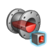
Box select all parts in the model to designate the Bounding
Solid domain.
Selected parts will turn red.
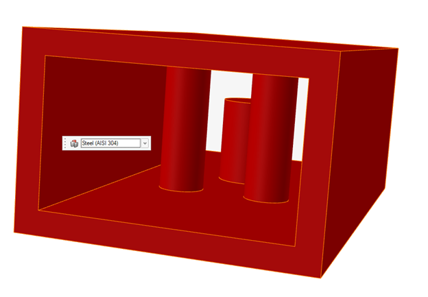
- In the microdialog, choose Steel (AISI 304) for the bounding solid domain.
-
Right-click and mouse through the check mark to exit, or
double-right-click.
The parts designated as Bounding Solid domains will turn black.
Create the Fluid Domain
-
Click the Create Fluid Domain icon.
A new fluid domain is detected and created.
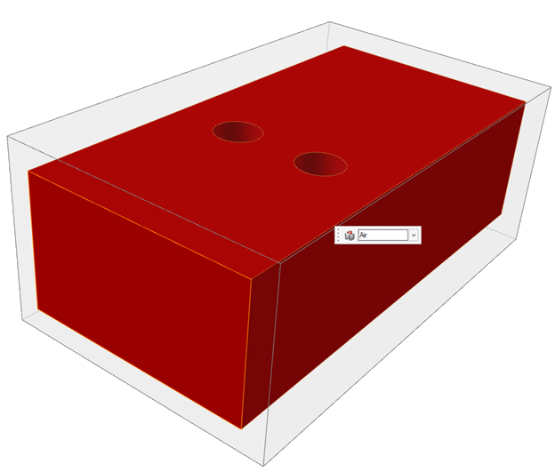
- In the microdialog, choose a fluid type.
-
Right-click and mouse through the check mark to exit, or
double-right-click.
The new fluid domain turns blue.
Designate Inlets
-
Select the Inlet icon.

-
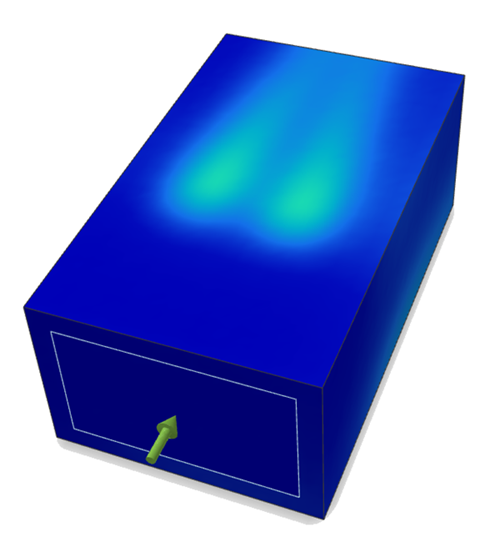
Select a face in the fluid domain where you would like to define an inlet. An
arrow appears at each defined inlet.
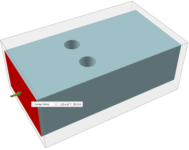
- In the microdialog, enter .25 m/s for the Average Velocity. Use the default value of 298.15 K for the temperature.
- Right-click and mouse through the check mark to exit, or double-right-click.
Designate Outlets
-
Click the Outlet icon.

-
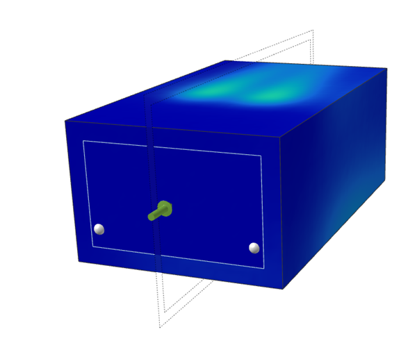
Select a face in the fluid domain where you would like to define an outlet.
An arrow appears at each defined outlet.
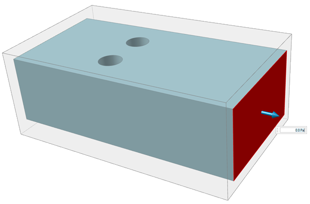
- Enter 0 Pa for guage pressure for the outlet face.
- Right-click and mouse through the check mark to exit, or double-right-click.
Define Thermal Conditions
-
Click the Face icon.

-
Select Solids.
Note: Ambient Temperature and Ambient HTC values can be changed as necessary. The default values are 293.15 K and 0 W/(m2*K). This option does not require any selection of parts or faces.
-
Select Component 1 and
Component
2 in the model.
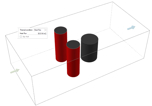 The microdialog appears with the following options:
- Temperature
- Convection
- Heat Flux
- Select the dropdown menu in the microdialog, then choose Heat Flux.
- Enter 50 W/m2 for the Heat Flux.
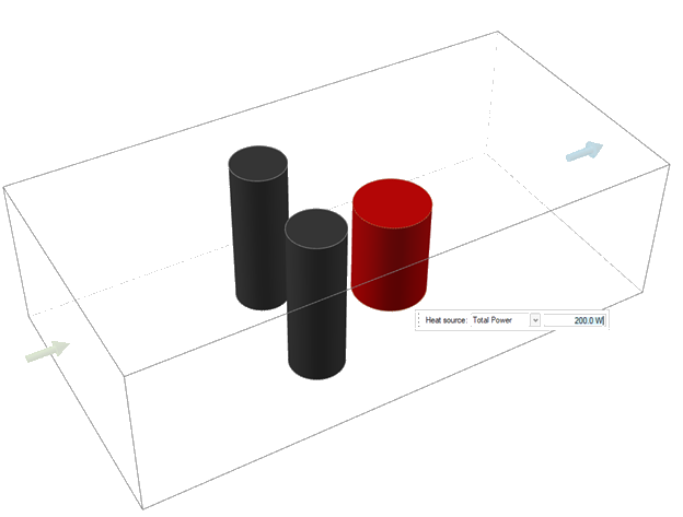
-
On the Fluids ribbon, select the
Part tool.
- Select Component 3.
- In the microdialog, select Total Power from the dropdown, and then enter 200.0 W.
-
In the guidebar, enter 298.15 K for Ambient
Temperature, and 25 W/(m2*K) for
Ambient HTC.
- Right-click and mouse through the check mark to exit, or double-right click.
Configure Solver Settings
-
Click the Custom Fluids Run icon.
- In the Simulation tab, set the Number of voxels to 100,000 and the Voxel size to .0023 m
-
Enable Compute thermal problem and
Include solids.
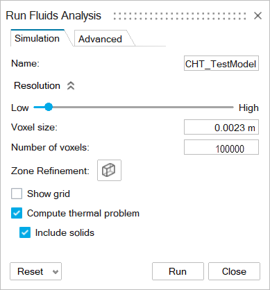
- Click Run.
Monitor Convergence Plots
While the analysis is running, monitor the convergence plots. The convergence
plots automatically appear after you click Run.
-
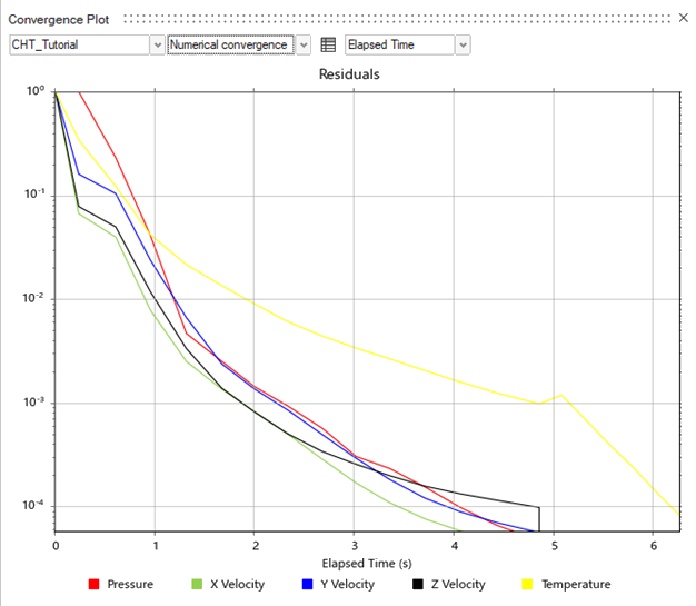
At the top of the Convergence Plots window, use
the dropdown menu to visualize the simulation data with
Engineering quantities or
Numerical convergence.
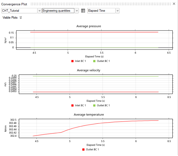
Additionally, you can select Show Convergence Table to visualize the result quantities in a table.

Review Simulation Results
-
Once the simulation is completed, a green flag appears in the
Analyze tool group.

-
Click the green flag to Import Completed Runs.
The results from the simulation will load in the modeling window.
-
Generate different result types using the Analysis
Explorer.
-
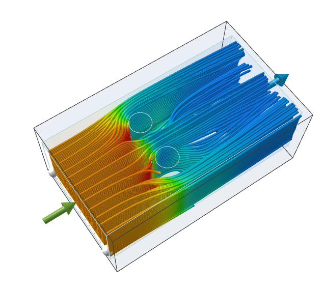
Click
 to visualize your results with
streamlines.
to visualize your results with
streamlines.
-
Click
-
Optionally, you can create local streamlines in the model:
-
Click
 to create the first linear streamline
region.
to create the first linear streamline
region.
-
Click to create the second linear streamline
region.
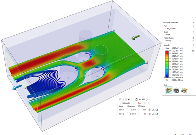
-
In the Analysis Explorer, change the Result Type to Velocity.
The model should look similar to the image below:
-
Click
-
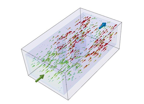
Click
 to visualize your results with vectors.
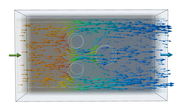
-
Under Result Types, use the dropdown menu to select
Velocity.
Results visualized as Velocity are displayed.
- Deselect Vectors as the result Style Option.
-
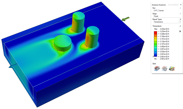
Under Result Types, use the dropdown menu to select
Temperature.
Results visualized as Temperature are displayed.
-
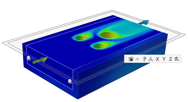
You can make a section cuts of the temperature results.
-
In the Object Browser, click
 to next to the component names to hide
Component 1, Component
2, and Component 3.
to next to the component names to hide
Component 1, Component
2, and Component 3.
-
In the bottom-left of the modeling window, select Section
Cuts
 .
.
-
In the microdialog, click
 .
.
-
Click the grey section cut pane.
-
In the Object Browser, click
 to next to the component names to
unhide Component 1, Component
2, and Component 3.
The components appear in the model.
to next to the component names to
unhide Component 1, Component
2, and Component 3.
The components appear in the model. -
Right-click and mouse through the check mark to exit, or double-right
click.
-
In the Object Browser, click