
Set Up and Run a Fluids Simulation
Run a Fluids simulation using default or custom settings.
Fluids Quick Run
Use the default settings to run a Fluids simulation for the selected parts.
-
On the Fluids ribbon, click the Fluids Quick Run
 button in the Analyze tool
group.
button in the Analyze tool
group. 
-
Let the analysis run to completion.
Tip: To find and open a tool, press Ctrl+F. For more information, see Find and Search for Tools.
Custom Fluids Run
Run a Fluids simulation with custom settings.
-
On the Fluids ribbon, click the Custom Fluids Run
 button in the Analyze tool
group.
button in the Analyze tool
group.
Tip: To find and open a tool, press Ctrl+F. For more information, see Find and Search for Tools. -
Customize the settings:
Table 1. Simulation tab Option Description Name Enter the name of the simulation. Resolution Drag the slider to the left for a fast, low-resolution simulation. Drag the slider to the right to increase the voxel resolution. Voxel size Define the size of the voxel mesh used for the calculation. Number of voxels Set the number of voxels to use in the simulation domain. Zone Refinement Click the  button, then
select a section of the part to create a zone on the part
where you would like to refine the mesh. Drag the arrows to
resize the refinement zone. Use the move tool to translate
or rotate the refinement zone. The microdialog controls the
refinement level. Level 1 will create
full-sized voxels. Level 2 will
create half-sized voxels. Each increasing level cuts the
voxel size in half. Greater refinement levels yield more
detailed results, but increased calculation time.
button, then
select a section of the part to create a zone on the part
where you would like to refine the mesh. Drag the arrows to
resize the refinement zone. Use the move tool to translate
or rotate the refinement zone. The microdialog controls the
refinement level. Level 1 will create
full-sized voxels. Level 2 will
create half-sized voxels. Each increasing level cuts the
voxel size in half. Greater refinement levels yield more
detailed results, but increased calculation time. Part Refinement Click the  button, then
select the part whose mesh you would like to refine. The
microdialog controls the refinement level.
button, then
select the part whose mesh you would like to refine. The
microdialog controls the refinement level. Wall Refinement Click the  button, then
select a part whose mesh you would like to refine in the
vicinity of its walls. The microdialog controls the
refinement level and the distance from the walls to which
the mesh will be refined.
button, then
select a part whose mesh you would like to refine in the
vicinity of its walls. The microdialog controls the
refinement level and the distance from the walls to which
the mesh will be refined. Show grid Turn on to show the grid that will be generated on the part side. Compute thermal problem Turn on to compute the temperature field in the simulation domain. Include Gravity Include Gravity is enabled by default if Variable Density is enabled in the fluid domain. Click the button to set the direction
of gravity.Note: If you disable Include Gravity, Variable Density will also be disabled.
button to set the direction
of gravity.Note: If you disable Include Gravity, Variable Density will also be disabled.Include solids Turn on to compute the temperature field in static and movable solids. Use symmetry Turn on to save simulation time by analyzing half of a symmetrical part. You can reorient and translate the plane of symmetry if necessary. Use RealTime Visualization If enabled, fluids analysis data can be displayed as soon as it is available rather than only after the entire analysis is complete. Note: This option is only supported when the simulation is performed on NVIDIA GPUs.Table 2. Advanced tab Option Description Termination criteria Stop the simulation when the selected criteria are met. - Physics: Stop the simulation
when the physics convergence criteria are met.
During the simulation, global engineering quantities such as flow velocities, pressures, flow rates, temperatures, heat fluxes, and forces are tracked on inlets, outlets, and surfaces with thermal conditions. Selecting Physics will terminate the simulation when these global quantities have reached stable values. Use this setting if the goal is to obtain good global estimates of engineering quantities.
- Equations: Stop the
simulation when the equations criteria are met.
During the simulation, the governing equations of fluid flow and heat transfer (pressure, x/y/z/ velocity components, and temperature) are solved in an iterative manner. The errors in the solution to these five equations are very high at the start of the simulation and gradually decrease as the simulation progresses. These errors are quantified and stored as "residuals." The starting values of the residuals are always 1.0 and are expected to decrease as the simulation progresses. The equations are considered to be solved with acceptable error when all five residual values drop below a value of 10-4. The Equations setting terminates the simulation when the residuals drop below 10-4. Sometimes, due to local flow instabilities, the equation residuals tend to stall at values higher than 10-4. In cases where the flowfield is unsteady by nature, it is impossible for the equations criteria to be satisfied since a stationary (steady-state) solution does not exist. This may result in the simulation running much longer than necessary. In such cases, it is more helpful to use the Physics option since small local oscillations often do not impact the global physics convergence.
- Physics or Equations: Stop the simulation when either the physics or equations criteria are met, whichever occurs first. In most practical scenarios, this is the recommended setting.
- Physics and Equations: Stop the simulation when both the physics and equations criteria are met. This is the most stringent requirement for convergence. Use this only when you want to ensure that the final results are absolutely converged in terms of both global and local solutions.
Output frequency steps Define the output frequency steps for the simulation. Max. time steps Define the maximum number of time steps allowed in the simulation. CFL Change the Courant–Friedrichs–Lewy number for the simulation. Greater CFL numbers yield fewer incremental updates to the simulation, making the simulation run more quickly. Typical range of CFL number that can be used are between 1 and 500. The default CFL number is set to 100. When using a lower CFL number, set a higher value for the number of maximum timesteps to achieve convergence. Note: High CFL numbers are not recommended for unsteady flows, such as in models with rotating components.Surface Monitor Request surface outputs on desired surfaces. You can obtain engineering data such as average pressure, velocity, temperature, flow rate, and forces on the specified surfaces. Flow type Select a flow type. - Turbulent
- LaminarNote: Fluid flows are commonly divided into two regimes: laminar and turbulent. Laminar flows are typically orderly and unidirectional in nature; turbulent flows are chaotic and multidirectional. A simple way to understand these two flow regimes is to observe water flowing from an open tap. When we open the tap at first, water comes out slowly as an orderly constrained tube. This is representative of a laminar flow. As we open the tap more, allowing the water to come out faster, we notice a visible disruption to the orderly flow tube previously observed. This chaotic stream is representative of a turbulent flow.
For a given fluid material and geometry, the higher the flow speed, the more turbulent the fluid flow is expected to be. This dependence on geometry, material properties, and flow speed are combined to create a nondimensional quantity called the Reynolds number. The Reynolds number is used to commonly categorize a specific flow condition as laminar or turbulent. For example, fluid flow through a circular pipe is expected to be laminar when the Reynolds number is less than 2000, and is considered fully turbulent at a Reynolds number of about 3500. Between these two values, the flow is considered transitional.
Select Turbulent when the fluid flow being simulated is expected to be turbulent in nature. This will activate the Spalart-Allmaras turbulence model with all-yplus wall-functions to model turbulent flows. Select Laminar if the flow is known to be laminar. If the exact flow regime being simulated is unknown or transitional, select Turbulent. The simulation will automatically apply the correct treatment based on the local flow speed.
Current GPU Currently selected GPU to run simulations (available when GPU solver type is selected) Validate GPU Check if a supported NVIDIA GPU is available to run the simulation. Improve convergence Turn on to activate the Algebraic Multigrid (AMG) linear solver to assist with simulation convergence difficulties. Note: To restore the default settings, click the Reset button and select Defaults. - Physics: Stop the simulation
when the physics convergence criteria are met.
- Click the Run button.
Run Status
View the status of the current run, as well runs for the current model that have not yet been viewed. To see all past runs, you need to view the run history.
-
Hover over the Analyze icon, then select the
Run Status tool.

Tip: To find and open a tool, press Ctrl+F. For more information, see Find and Search for Tools.The run status window is displayed.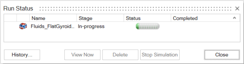
- Optional: You can view a simulation's data in real time as it becomes available. In the run status window, select the run and click the View Now button. The analysis explorer will open and populate with simulation data as it becomes available.
-
When the run is complete, review its status.
Status Description Note 
The run completed successfully. This is also indicated by a green flag above the Analyze icon. You can click the green flag to display the results. 
The run was incomplete. If running an analysis, the run was incomplete. Some but not all of the result types may be available. You should run a new analysis to generate complete results.
If running an optimization, the run was completed but with warnings or violations. Double-click the name of the run in the Run Status dialog, and then click the Design Violations button in the Shape Explorer for more information.

The run failed and no meaningful results are available. This is also indicated by a red flag above the Analyze icon. -
View one or more runs.
- To view a run, double-click the row.
- To view multiple runs, hold down Ctrl or
Shift while clicking the rows, and then click
the View Now button.Note: If several runs are associated with the same part, the result from the most recently completed run for that part will be activated in the modeling window.
- To open the directory where a run is stored, right-click the run name and select Open Run Folder.
- To view deleted or previously viewed runs, click the History button.
- To delete a run, select the run and press Delete. You can also delete runs using the right-click context menu in the Analysis Explorer and the Model Browser.
Run History
View, sort, open, and delete past runs for the current and previous models.
-
Hover over the Analyze or Analyze
Fluids icon, then select the Run
Status tool.

Tip: To find and open a tool, press Ctrl+F. For more information, see Find and Search for Tools.The run history is displayed.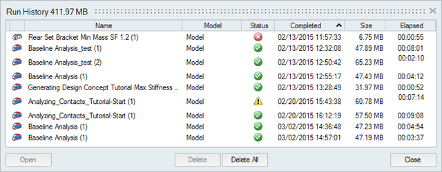
-
Review the status of the run.
Status Description Note 
The run completed successfully. 
The run was incomplete. If running an analysis, the run was incomplete. Some but not all of the result types may be available. You should run a new analysis to generate complete results.
If running an optimization, the run was completed but with warnings or violations. Double-click the name of the run in the Run Status dialog, and then click the Design Violations button in the Shape Explorer for more information.

The run failed and no meaningful results are available. - To view a run, double-click the row.
- To open the directory where a run is stored, right-click the run name and select Open Run Folder. The default directory where the run history is stored can be changed in the Preferences under Run Options.
- By default, you will receive a notification when the run history exceeds a certain size. You can change the size limit or turn off the notification in the Preferences under Run Options.
- To delete a run, select the run and press Delete.