
Runtime Monitoring
OptiStruct currently supports monitoring functionality for Small and Large Displacement Nonlinear static, Large Displacement Nonlinear Transient Analysis, and Fluid-Structure Analysis. Additionally, monitoring is also supported for Nonlinear Optimization runs.
The following sections provide specific information regarding the procedure for runtime monitoring.
Monitor Nonlinear Structural Analysis and Structural FSI
- .out file
Regular ASCII .out file, and it is a powerful basic monitoring tool as well. This is output on-the-fly by default for any OptiStruct run.
- _nl.h3d file
Dedicated nonlinear monitoring H3D file which contains displacements only results. In addition, this also contains Grid Sets identifying contact status changes and Element Sets which identify distorted elements. This is output on-the-fly when NLMON Bulk/Subcase pair is specified.
- _nl.out file
Dedicated nonlinear monitoring ASCII out file which contains specialized nonlinear solution information. This is output on-the-fly by default for any nonlinear run. In addition, this file also contains a summary of contact status change grids and distorted elements. This output can be controlled via the NLPRINT Bulk/Subcase Entry pair. This file is output on-the-fly when NLMON Bulk/Subcase pair is specified.
- .monitor file
Dedicated nonlinear monitoring ASCII file which contains specialized nonlinear solution information. This is output on-the-fly by default for any nonlinear run.
- _ld.monitor file
Dedicated nonlinear monitoring ASCII file which contains specialized nonlinear solution information. This is output on-the-fly by default for any nonlinear run.
- _impl.h3d file
General on-the-fly nonlinear output file for implicit nonlinear runs. This is output on-the-fly when NLOUT Bulk/Subcase pair is specified in conjunction with PARAM,IMPLOUT,YES or if NLOUT argument on specific I/O Entries is specified pointing to NLOUT Bulk Data. The _impl.h3d file is not specifically a dedicated nonlinear debugging tool but it can be used to visualize results on-the-fly for nonlinear runs too.
- _e.out file
Dedicated ASCII file for monitoring Energy output from Nonlinear Analysis. This is output on-the-fly for a Nonlinear OptiStruct run if the NLENRG Bulk/Subcase entry pair is specified.
- _e.nlm file
Dedicated HyperGraph data file for monitoring Energy output from Nonlinear Analysis. The global energy output on-the-fly for each increment of a nonlinear OptiStruct run, is output, by default for all subcases in the _e.nlm file. Frequency-control and entity-based output can be activated for energy output using the NLENRG Bulk/Subcase Entry pair.
The _nl.out file and the _nl.h3d file can be used in conjunction with the os_out_file_parser.tcl script in HyperView to visualize nonlinear convergence progress and perform detailed nonlinear debugging. The process to accomplish this is illustrated below.
Two files are required for this, the <filename>_nl.h3d file, and additionally convergence table information for the specified intervals which is output to the _nl.out file. The convergence table information is currently only supported for Large Displacement Nonlinear Analysis.
If the INT field is set to INC, then you can monitor the progression of the model through the nonlinear run by loading the <filename>_nl.h3d file in HyperView during runtime and looking at the results.
To monitor and debug the model at each iteration (in every increment), you should set the INT field to ITER (or use PARAM,NLMON,DISP). For the case where the INT field is set to ITER, you can debug the model by going through the following steps:
-
Add NLMON Bulk Data Entry and NLMON
Subcase Information Entry pair to the corresponding Nonlinear subcase (with
INT field set to ITER) for which the
results monitoring and debugging is required (you can also use
PARAM,NLMON instead).
The Bulk Data/Subcase pair overrides PARAM,NLMON, if both are specified).
-
Run the model.
A second H3D file named <filename>_nl.h3d will appear in your working directory.
-
Open HyperView and load the
<filename>_nl.h3d file result file.
The model results in HyperView appear at this point.
- Import the Tcl script. The script is located in the installation at: <install_directory>/altair/hwsolvers/scripts/os_out_file_parser.tcl
- Click and select the os_out_file_parser.tcl script and click Open.
-
In the subsequent OptiStruct OUT File Parser window,
select <filename>_nl.out from your working directory for
the Out File field.
Figure 1. 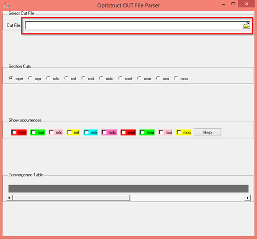
-
Click Open.
The monitored results are now loaded into the window.
Figure 2. 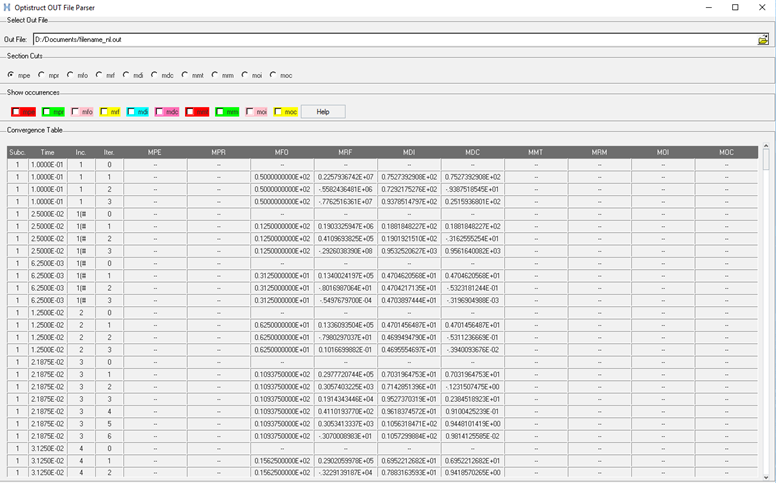
-
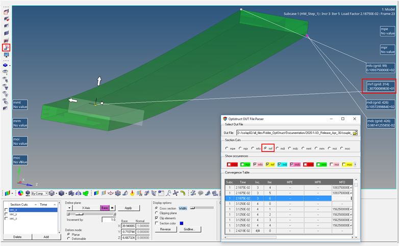
Activate the checkbox of the result type whose peak value occurrence you want
to investigate and click on the corresponding Iteration in the Convergence
table.
The corresponding grid point at which the result type attains its peak value is displayed in the Graphics Browser of HyperView.
Figure 3. 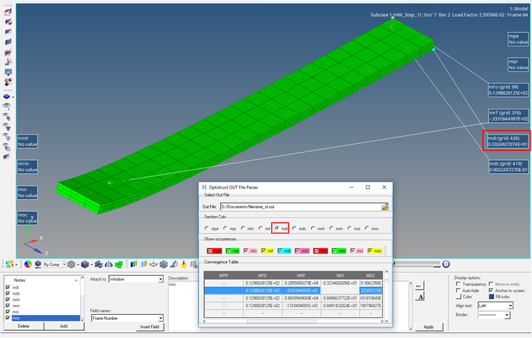
For more information on Nonlinear Analysis, refer to Nonlinear Static Analysis, Nonlinear Transient Analysis, and Structural Fluid-Structure Interaction Analysis.
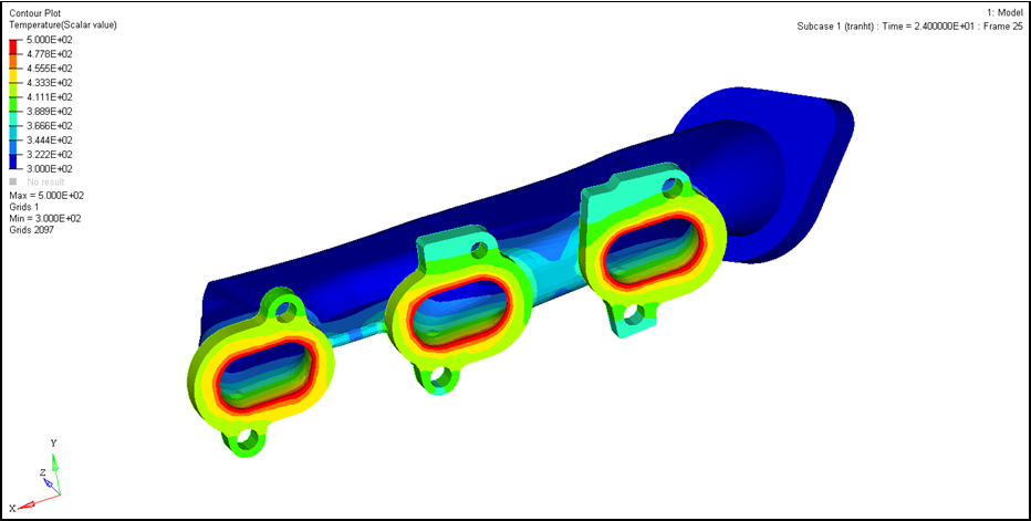
Thermal Fluid-Structure Interaction (Thermal FSI) Monitoring
During Thermal FSI Analysis, for the Structural Transient Heat Transfer solution, monitoring results are available by default at runtime, in the <filename>_ht.h3d file. This H3D file can be viewed in HyperView during runtime to monitor temperature results for each time-step.
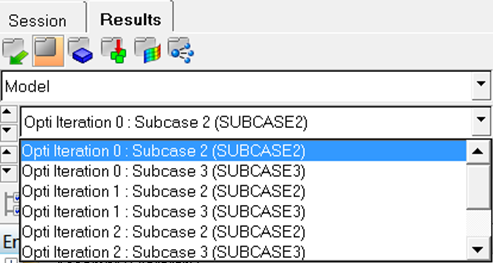
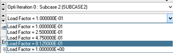
Nonlinear Optimization Monitoring
During Nonlinear Optimization, nonlinear results for each load increment is available for each optimization iteration.
Plot Convergence During Analysis
The convergence plot can be obtained for all nonlinear iterations across all subcases for nonlinear static and nonlinear transient analysis, using the Altair Compute Console (ACC).
The progress can also be monitored for all the optimization iterations.
To obtain the convergence plot:
-
Select the checkbox next to Use solver control and click
Run.
-
Click Graph to obtain the convergence plot, once the
analysis iterations begin.
Figure 9. 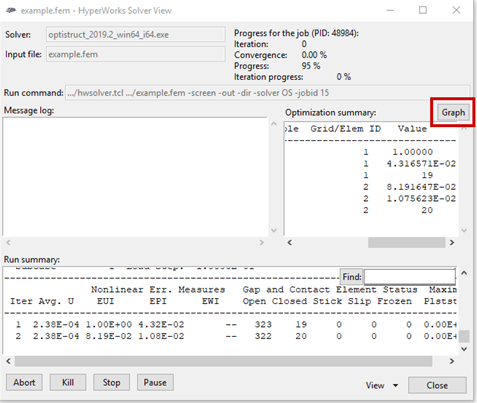
Figure 10. Convergence Plot Example 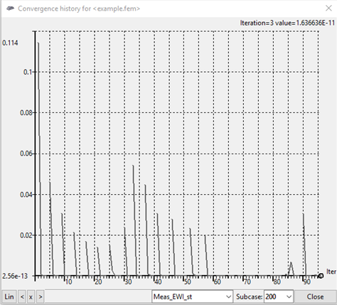
The drop-down options in the lower-right corner can be used to select the type of convergence plot and the subcase.
The different measures for convergence plots (force, displacement, and work) can be chosen from the drop-down menu. In addition, the gap close status can also be monitored in case of contact analysis
The toggles in the lower-left corner allow switching between log and linear scales and zooming the plot to the left or to the right edge of the plot.