Phase 2: Design Fine Tuning
Import and Review the Model
At the end of Phase 1, OptiStruct automatically created a new file, controlarm_lattice.fem, from your original optimization model. In this model, the original designable elements with a density below LB have been removed, those above UP remain unchanged and those in-between, are replaced by beam elements (CBEAM) representing the lattice structure.
The second phase of this optimization will optimize the radius of each joint in the lattice structure to determine where there is a need for material. The necessary design variables (DESVAR) and design variable property relationships (DVPREL1), along with the stress constraints are automatically created. In many cases, the model can be run as is, but it is advised to always review the optimization setup.
- Click .
- Select the controlarm_lattice.fem file.
- Click Open.
-
Review the model.
-
The beginning of the deck shows that the new file has retained your
original objective but added a new optimization parameter indicating
that this size optimization is Phase 2 of a lattice structure
optimization.
Figure 1. 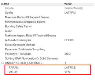
-
OptiStruct has inserted the
CBEAM elements, which represent the new lattice
material.
Figure 2. 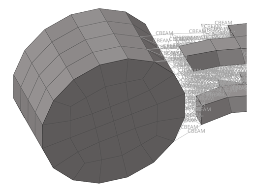
-
Each joint between multiple CBEAM elements has a
design variable created for it.
Figure 3. 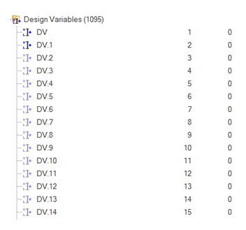
-
The design variable property relationships (DVPREL1)
are created, which relate properties to their associated design variable
for the size optimization in the second phase. These are followed by the
responses, the constraints, and the objective.
Note: The volume fraction response in the original model has been replaced by total volume in the size optimization phase, which will now be minimized and a new response has been added to constrain the von Mises stress in the lattice region to 200. This was created from the value in the last field of the LATTICE continuation card in the first phase.
Figure 4. 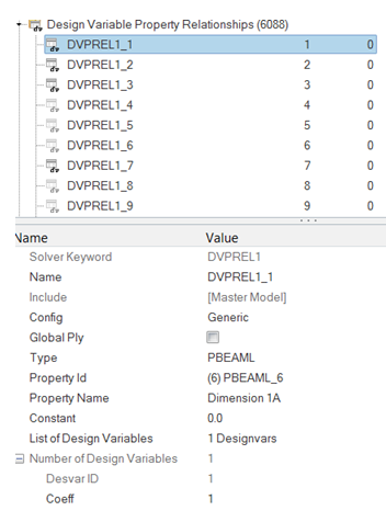
Figure 5. 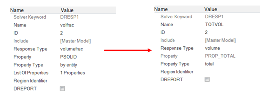
-
The beginning of the deck shows that the new file has retained your
original objective but added a new optimization parameter indicating
that this size optimization is Phase 2 of a lattice structure
optimization.
- Close the controlarm_lattice.fem file.
Run the Optimization
- Open the Compute Console (ACC).
- In the Input file(s) field, load the controlarm_lattice.fem file.
-
Click Run to run the optimization.
- When the optimization has completed, open the controlarm_lattice.fem file in a text editor to review critical information about the optimization run.
-
Verify that the optimization is fully converged and that the constraint is
satisfied.
Figure 7. 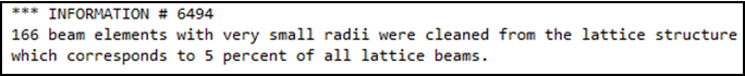
The difference in lattice penalty (lower than 1.8, set by the optimization parameters) causes the compliance of the final Phase 1 model to differ from the initial Phase 2 model. This compliance difference is also affected by solid elements retained in the Phase 2 model, which recover their full density/stiffness. For this reason, post-processing a lattice optimization requires that you analyze changes to the model compliance between the Phase 1 final optimization compliance and the Phase 2 initial compliance calculation and again at the end of Phase 2. - Open the Compute Console (ACC).
- Load the controlarm_lattice_optimized.fem file.
-
Click Run for verification purposes.
Since the optimization removes CBEAM elements of small radius after the last optimization, the compliance for the last optimized run should be confirmed against the controlarm_lattice_optimized.fem file, an analysis of the optimized structure provided by OptiStruct.
-
Compare the final compliance between the controlarm_lattice.out and controlarm_lattice_optimized.out files.
Figure 9. Final Compliance from the Optimization Run 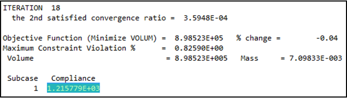
Figure 10. Final Compliance from the Analysis Model 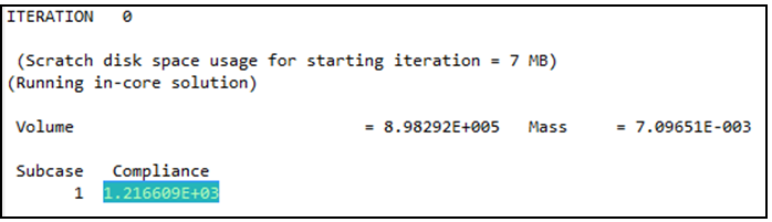
Post-process the Results
- Open HyperMesh Desktop.
- Import the file controlarm_lattice_optimized.fem into a new session.
-
On the Visualization toolbar, from the 1D Element Representation menu, select
1D Detailed Element Representation.
The CBAR elements in the model with their radii applied display.
Figure 11. View of the Optimized Solid/Lattice Model 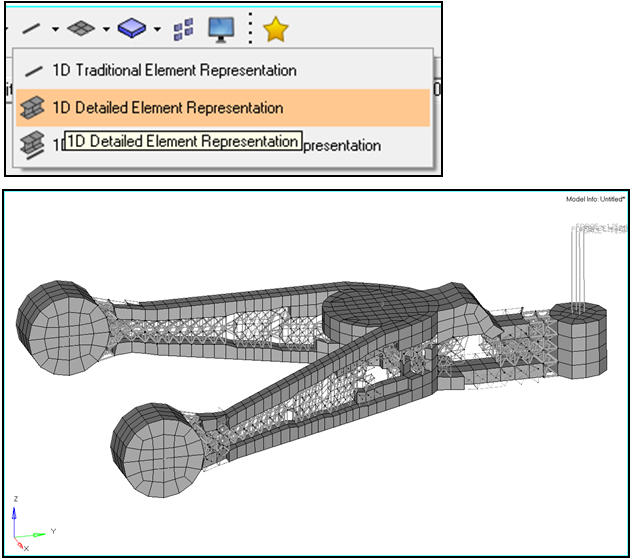
Figure 12. Front View of the Optimized Lattice/Solid Model Showing the Variation in CBAR Radius 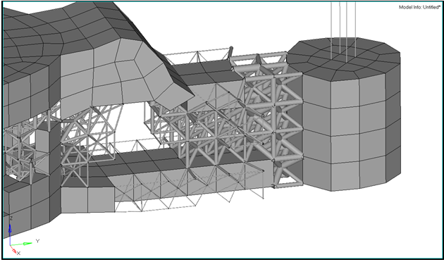
- In a new HyperView session, load the file controlarm_lattice_s1.h3d.
-
Edit visualization options.
- From the menu bar, click .
- In the Options dialog, select the Visualization section.
- Select Enable element marks.
- Set the BAR representation to Cylinder.
- In the Size of mark (model %), enter 0.125.
- Click Apply.
- Click OK.
Figure 13. 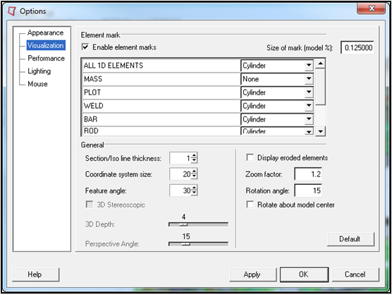
-
On the Results toolbar, click
 to open the
Contour panel.
to open the
Contour panel.
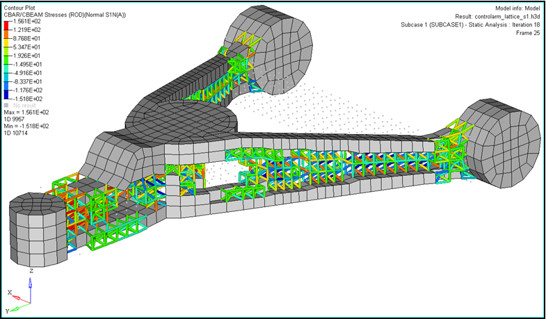
- Set the type to CBAR/CBEAM Stresses (ROD).
- Set the Subtype to NORMAL S1N(A).
-
Click Apply.
The beam element visualization is contoured.
Figure 14. Iteration 0 (Initial Sizing Design) 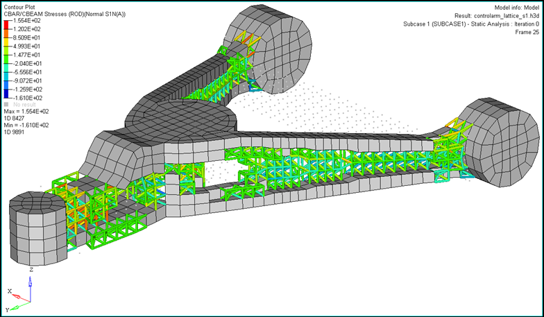
Figure 15. Last Iteration (Final Design)