OS-T: 1910 Dynamic Analysis of a Slider Crank with Flexible Connecting Rod
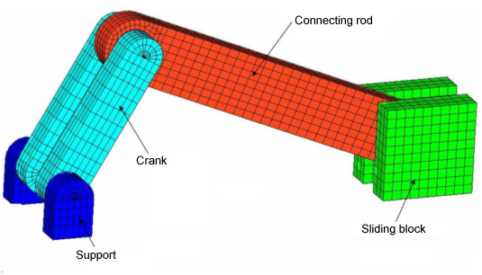
In this tutorial you will work with a slider crank model, which consists of a rigid crank, a flexible connecting rod, and a rigid sliding block. The objective of this analysis is to determine the deformation and stress of a flexible connecting rod under the high speed motion of the system.
This tutorial includes the creation of PRBODY (rigid body definition), PFBODY (flexible body definition), and JOINT in HyperMesh.
Launch HyperMesh and Set the OptiStruct User Profile
-
Launch HyperMesh.
The User Profile dialog opens.
-
Select OptiStruct and click
OK.
This loads the user profile. It includes the appropriate template, macro menu, and import reader, paring down the functionality of HyperMesh to what is relevant for generating models for OptiStruct.
Open the Model
- Click .
- Select the slider_crank.hm file you saved to your working directory.
-
Click Open.
The slider_crank.hm database is loaded into the current HyperMesh session, replacing any existing data.
Set Up the Model
Create PRBodies
- From the Analysis page, click the bodies panel.
- Select the create subpanel.
-
Define PRBODY for the support component.
- In the body= field, enter support.
- Click type= and select PRBODY.
- Using the props selector, select support.
- Click create.
-
Define PROBDY for the crank component.
-
Using the nodes selector, select the node (ID 25231) at the center of
RBE2 spider between connecting rod and crank.
Figure 2. 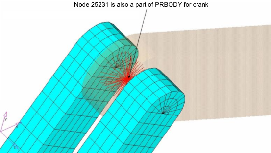
-
Using the nodes selector, select the node (ID 25231) at the center of
RBE2 spider between connecting rod and crank.
-
Define PROBDY for the block component.
-
Using the nodes selector, select the node (ID 25232) at the center of
RBE2 spider between connecting rod and block.
Figure 3. 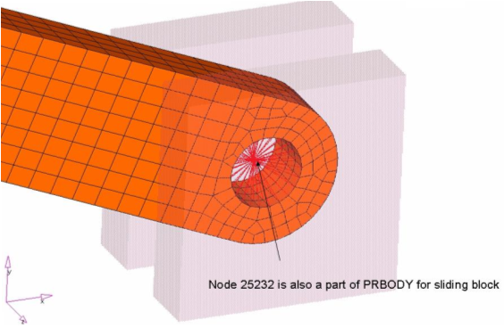
-
Using the nodes selector, select the node (ID 25232) at the center of
RBE2 spider between connecting rod and block.
- Click return.
Create Flex Bodies (PFBODY)
- From the Analysis page, click the bodies panel.
- Select the create subpanel.
- In the body= field, enter Rod.
- Click type= and select PFBODY.
- Using the props selector, select Rod.
-
Using the elems selector, select two RBE2 elements that are inside a hole on
the connecting rod.
Tip: You could also use 'elems by id' and input the IDs 18795 and 18796 to select the two RBE2 elements.
Figure 4. 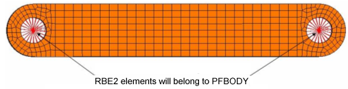
- Set CMS Method to Craig-Bampton.
-
Toggle number of modes to nmodes=, and enter
10.
Figure 5. 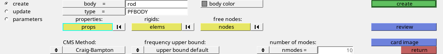
- Click create.
- Click return.
Create Joints
| Type of Joint | Removes Translational dof | Removes Rotational dof | Removes Total Number of dof |
|---|---|---|---|
| Revolute | 3 | 2 | 5 |
| Fixed | 3 | 3 | 6 |
| Translational | 2 | 3 | 5 |
-
Create the component, joints.
-
From the menu bar, click .
The Joints panel opens.
-
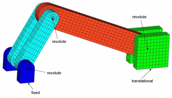
Create the fixed joint between ground and support.
Figure 7. 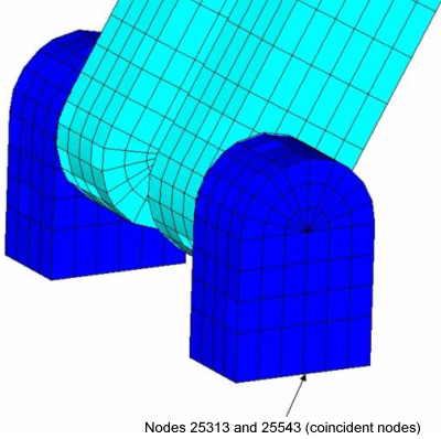
-
Create the revolute joint between support and crank.
Figure 8. 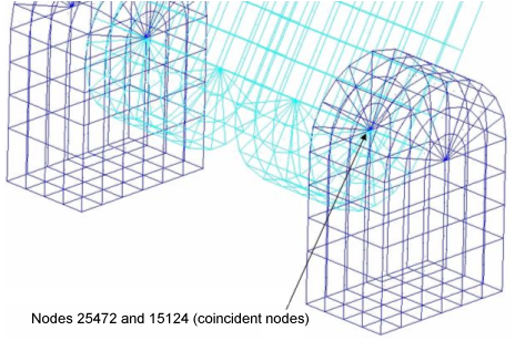
-
Create the revolute joint between the crank and connecting rod.
Figure 9. 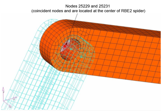
-
Create the revolute joint between the connecting rod and sliding block.
Figure 10. 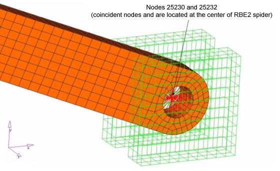
-
Create the translational joint between the sliding block and ground.
Figure 11. 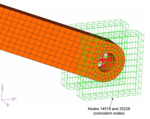
- Click return.
Create DTI, UNITS
- From the menu bar, click to open the Control Cards panel.
- Click DTI_UNITS.
-
Define the unit system, as shown in Figure 12.
Figure 12. 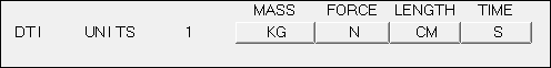
- Click return twice to return to the main menu.
Create Load Collectors
In this step you will create the gravity force that applies to the model and MBSIM Bulk Data card, which is to specify the parameter for multibody simulation.
-
In the Model Browser, right-click and select from the context menu.
A default load collector displays in the Entity Editor.
- For Name, enter SIM.
- Click Color and select a color from the color palette.
- Set Card Image to MBSIM and click Close.
-
Input the values as illustrated below.
Figure 13. 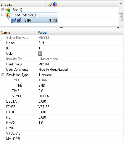
-
Create another load collector.
-
Input the values as illustrated below.
Figure 14. 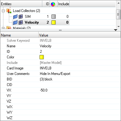
-
Input the values as illustrated below.
Create Load Steps
- In the Model Browser, right-click and select from the context menu.
- For Name, enter Dynamic.
- Set Analysis type to Multibody dynamics.
-
Define MBSIM.
-
For MBSIM, click Unspecified >
 to open Advanced Selection.
- In the dialog, select SIM and click OK.
-
For MBSIM, click Unspecified >
- In Subcase Options, select .
-
For INVEL, click Unspecified > to open Advanced Selection.
- In the dialog, select Velocity and click OK.
Submit the Job
-
From the Analysis page, click the OptiStruct
panel.
Figure 15. Accessing the OptiStruct Panel 
- Click save as.
-
In the Save As dialog, specify location to write the
OptiStruct model file and enter
slider_crank_complete for filename.
For OptiStruct input decks, .fem is the recommended extension.
-
Click Save.
The input file field displays the filename and location specified in the Save As dialog.
- Set the export options toggle to all.
- Set the run options toggle to analysis.
- Set the memory options toggle to memory default.
- Click OptiStruct to launch the OptiStruct job.
- slider_crank_complete_mbd.abf
- Binary plotting file.
- slider_crank_complete_mbd.h3d
- Binary results file (Modal results).
- slider_crank_complete_mbd.log
- Log file from OS-Motion containing the information on the joints and markers, simulation etc., which are specific to MBD analysis.
- slider_crank_complete_mbd.mrf
- Binary results file for plotting.
- slider_crank_complete_mbd.xml
- Model file in .xml format – solver intermediate input deck.
View the Results
In this step you will view the results in HyperView, which will be launched from within the OptiStruct panel of HyperMesh.
HyperView is a complete post-processing and visualization environment for finite element analysis (FEA), multibody system simulation, video and engineering data.
-
From the OptiStruct panel of the Analysis page,
click HyperView.
The path and filename for slider_crank_complete.h3d appears in the fields to the right of Load model and Load results. This is fine because the .h3d format contains both model and results data.
The model and results are loaded in the current HyperView window.
-
Click the Contour panel toolbar icon
 .
.
- Under Results type: select Displacement(v).
- Click Apply.
-
Start/stop the animation using the Animation Controls in the panel next to the
playback controls.
Figure 16. 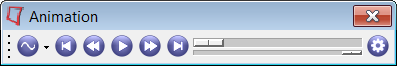
-
Verify Animate Mode is set to
 (Transient).
- Click the Start/Pause Animation icon to start the animation.
- With the animation running, use the bottom slider bar to adjust the speed of the animation.
- Click the Start/Pause Animation icon again to stop the animation.
Figure 17. 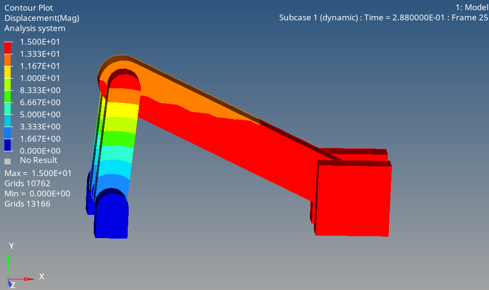
-
Verify Animate Mode is set to
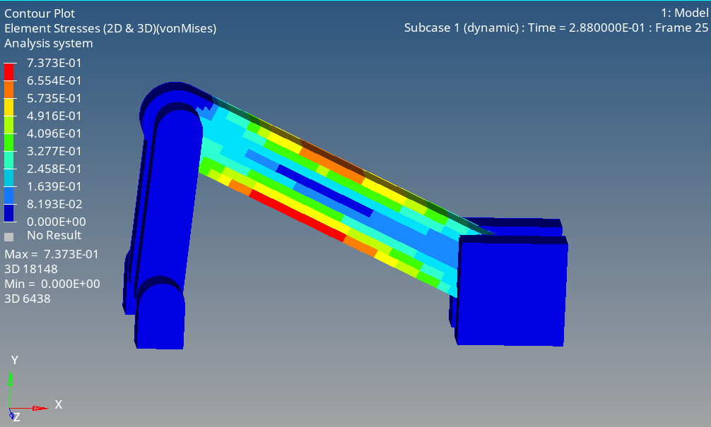
- In the Contour panel, under Results type, select Element Stresses [2D & 3D].
- Set Stress type to von Mises.
- Click Apply.
-
Click the Start/Pause Animation icon to start the
animation.
Figure 18.