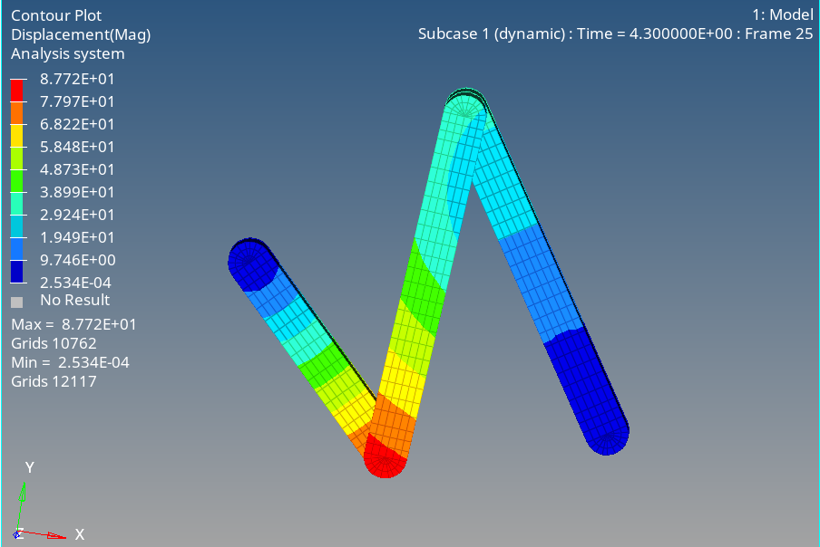
OS-T: 1900 Dynamic Analysis of a Three-body Model
In this tutorial, dynamic analysis on a simple three rigid bodies model is performed using OptiStruct. The force of gravity acts along the global Y axis, and the system has one degree of freedom.
Launch HyperMesh and Set the OptiStruct User Profile
-
Launch HyperMesh.
The User Profile dialog opens.
-
Select OptiStruct and click
OK.
This loads the user profile. It includes the appropriate template, macro menu, and import reader, paring down the functionality of HyperMesh to what is relevant for generating models for OptiStruct.
Open the Model
- Click .
- Select the 3bodies_dynamics.hm file you saved to your working directory.
-
Click Open.
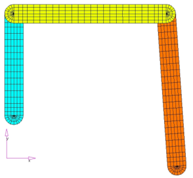
The 3bodies_dynamics.hm database is loaded into the current HyperMesh session, replacing any existing data. The model has three components and a few free nodes that will be used to create bodies and joints for the MBD model.
Set Up the Model
Create PRBodies
- From the Analysis page, click the bodies panel.
- Select the create subpanel.
-
Define PRBODY for the body1 component.
- In the body= field, enter blue.
- Click type= and select PRBODY.
- Using the props selector, select body1.
- Click create.
-
Define PROBDY for the body2 component.
- In the body= field, enter lime.
- Click type= and select PRBODY.
- Using the props selector, select body2.
- Click create.
-
Define PROBDY for the body3 component.
- In the body= field, enter orange.
- Click type= and select PRBODY.
- Using the props selector, select body3.
- Click create.
- Click return.
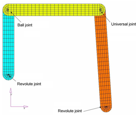
Create Joints
You will create two revolute joints, one ball joint, and one universal joint to constrain the degrees of freedom, such that the remaining degree of freedom will be just 1.
| Type of Joint | Removes Translational dof | Removes Rotational dof | Removes Total Number of dof |
|---|---|---|---|
| Revolute | 3 | 2 | 5 |
| Universal | 3 | 1 | 4 |
| Ball (Spherical) | 3 | 0 | 3 |
-
Create the component, joints.
-
From the menu bar, click .
The Joints panel opens.
-
Create the revolute joint at the lower right corner of body3.
-
Click create.
The vectors 12319 to 12910 define the axis of rotation of the revolute joint.
Figure 3. 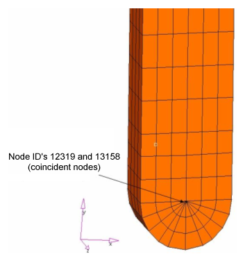
-
Click create.
-
Create the revolute joint at the lower left corner of body1.
- Select node ID 11115 as the first terminal and node ID 13159 as the second terminal.
- Select node ID 11706 as a node for first orientation.
- Click create.
The vectors 11115 to 11706 define the axis of rotation of the revolute joint.Figure 4. 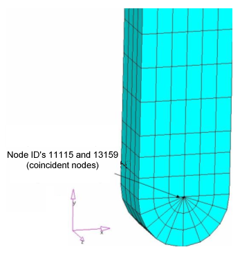
-
Create the universal joint between body3 and body2.
- Set joint type to universal.
- Select node ID 12330 as first terminal which belongs to body3, and select node ID 7589 as second terminal which belongs to body2.
- Select node ID 12921 as a node for first orientation, and select node ID 11944 as a node for second orientation.
- Click create.
The vectors 12330 to 12921 define the first cross pin axis, and the vectors 7589 to 11944 define second cross pin axis.Figure 5. 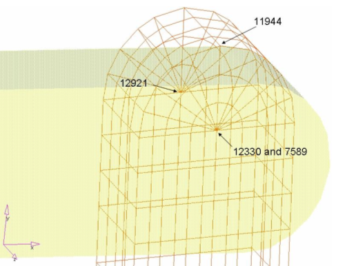
-
Create a ball (spherical) joint between body1 and body2.
- Set joint type to ball.
- Select node ID 11104 as first terminal which belongs to body1, and select node ID 7578 as second terminal which belongs to body2.
- Click create.
Figure 6. Ball Joint between body1 and body2 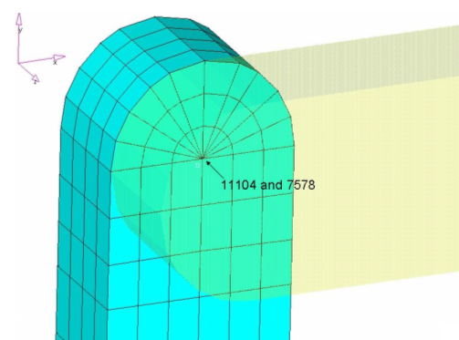
Apply Loads and Boundary Conditions
The gravity force that applies to the model and MBSIM Bulk Data card, which is to specify the parameter for multi body simulation, is created in the following steps.
Create Load Collectors
In this step you will create the gravity force that applies to the model and MBSIM Bulk Data card, which is to specify the parameter for multibody simulation.
-
In the Model Browser, right-click and select from the context menu.
A default load collector displays in the Entity Editor.
- For Name, enter gravity.
- Click Color and select a color from the color palette.
- Set Card Image to GRAV and click Close.
-
Input the values as illustrated below.
Figure 7. 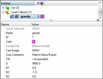
-
Create another load collector.
-
Input the values as illustrated below.
Figure 8. 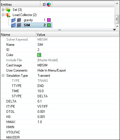
-
Input the values as illustrated below.
Create Load Steps
- In the Model Browser, right-click and select from the context menu.
- For Name, enter Dynamic.
- Set Analysis type to Multi-body dynamics.
-
Define MLOAD.
-
For MLOAD, click Unspecified >
 to open Advanced Selection.
- In the dialog, select gravity and click OK.
-
For MLOAD, click Unspecified >
- In Subcase Options, select .
-
For MBSIM, click Unspecified > to open Advanced Selection.
- In the dialog, select SIM and click OK.
Submit the Job
-
From the Analysis page, click the OptiStruct
panel.
Figure 9. Accessing the OptiStruct Panel 
- Click save as.
-
In the Save As dialog, specify location to write the
OptiStruct model file and enter
3bodies_dynamics_complete for filename.
For OptiStruct input decks, .fem is the recommended extension.
-
Click Save.
The input file field displays the filename and location specified in the Save As dialog.
- Set the export options toggle to all.
- Set the run options toggle to analysis.
- Set the memory options toggle to memory default.
- Click OptiStruct to launch the OptiStruct job.
View the Results
In this step you will view the results in HyperView, which can be launched from within the OptiStruct panel of HyperMesh.
HyperView is a complete post-processing and visualization environment for finite element analysis (FEA), multi-body system simulation, video and engineering data.
-
While in the OptiStruct panel of the Analysis page,
click HyperView.
- Optional: If a window appears with a warning message, click OK.
The path and file name for 3bodies_dynamics_complete.h3d appears in the fields to the right of Load model and Load results. This is fine because the .h3d format contains both model and results data.
The model and results are loaded in the current HyperView window.
-
Click
 to open the Contour panel.
- Under Results type, select Displacement(v).
- Click Apply.
-
Start/stop the animation using the Animation Controls in the panel next to the
playback controls.
Figure 10. 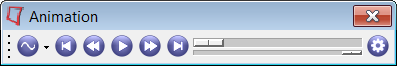
-
Verify Animate Mode is set to
 (Transient).
- Click the Start/Pause Animation icon to start the animation.
- With the animation running, use the bottom slider bar to adjust the speed of the animation.
- Click the Start/Pause Animation icon again to stop the animation.
-
Verify Animate Mode is set to