Phase 1: Reference Design Synthesis (Free-Size Optimization)
In free-size optimization, the thickness of each designable element is defined as a design variable. Applying this concept to the design of composites implies that the design variables are the thickness of each Super-ply (total designable thickness of a ply orientation) per element.
The following optimization setup is defined in the concept design phase to identify
the stiffest design for the given fraction of the material. To obtain more
meaningful results, manufacturing constraints are incorporated and carried through
all design phases automatically.
- Objective
- Minimize the weighted compliance of the two load cases.
- Constraints
- Volume fraction < 0.3
- Design Variables
- Element thicknesses of each ply orientation.
- Manufacturing Constraints
- Ply percentage for the 0s no more than 80% exist.
Launch HyperMesh and Set the OptiStruct User Profile
-
Launch HyperMesh.
The User Profile dialog opens.
-
Select OptiStruct and click
OK.
This loads the user profile. It includes the appropriate template, macro menu, and import reader, paring down the functionality of HyperMesh to what is relevant for generating models for OptiStruct.
Import the Model
-
Click .
An Import tab is added to your tab menu.
- For the File type, select OptiStruct.
-
Select the Files icon
 .
A Select OptiStruct file browser opens.
.
A Select OptiStruct file browser opens. - Select the fairing.fem file you saved to your working directory.
- Click Open.
- Click Import, then click Close to close the Import tab.
Set Up the Optimization
Create Free-size Optimization Design Variables
- From the Analysis page, click the optimization panel.
- Click the free size panel.
-
Create the design variable fairing.
- Select the create subpanel.
- In the desvar= field, enter fairing.
- Set type to PCOMP(G).
- Using the props selector, select fairing_ply.
- Click create subpanel.
The design variable fairing is created for the free-size optimization. -
Define the manufacturing constraints on ply percentage and ply balance.
-
Define the PLYPCT, BALANCE and PLYMAN constraints as shown in Figure 1.
Figure 1. DSIZE Data Entry Fields 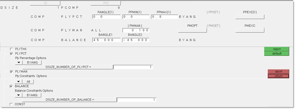
-
Define the PLYPCT, BALANCE and PLYMAN constraints as shown in Figure 1.
- Click return and go back to the Optimization panel.
Create Optimization Responses
- From the Analysis page, click optimization.
- Click Responses.
-
Create the volume fraction response.
- In the responses= field, enter Volfrac.
- Below response type, select volumefrac.
- Set regional selection to total and no regionid.
- Click create.
-
Create the weighted component response.
- In the responses= field, enter wcomp.
- Below response type, select weighted comp.
- Click loadsteps, then select all loadsteps.
- Change the weighting factors for gravity and pressure to 1.0.
- Click return.
- Click create.
- Click return to go back to the Optimization panel.
Create Design Constraints
- Click the dconstraints panel.
- In the constraint= field, enter con_vol.
- Click response = and select volfrac.
- Check the box next to upper bound, then enter 0.3.
- Click create.
- Click return to go back to the Optimization panel.
Define the Objective Function
- Click the objective panel.
- Verify that min is selected.
- Click response= and select wcomp.
- Click create.
- Click return twice to exit the Optimization panel.
Define the Output Request
- From the Analysis page, click the control cards panel.
-
Define the GLOBAL_OUTPUT_REQUEST card.
-
Click return.
Figure 2. Request CSTRAIN and CSTRESS Results Output to the .h3d File 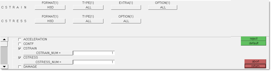
-
Click return.
-
Define the OUTPUT card.
- Click OUTPUT.
- In the number_of_outputs field, enter 1.
- Set KEYWORD to FSTOSZ.
- Set FREQ to YES.
- Click return.
OptiStruct automatically generates a sizing model after free-size optimization.Figure 3. Request the Free-size to Size (FSTOSZ) Optimization Output File for Phase 2 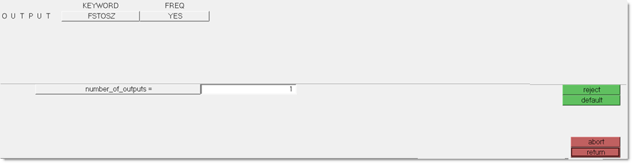
Run the Optimization
- From the Analysis page, click OptiStruct.
- Click save as.
-
In the Save As dialog, specify location to write the
OptiStruct model file and enter
fairing_freesize for filename.
For OptiStruct input decks, .fem is the recommended extension.
-
Click Save.
The input file field displays the filename and location specified in the Save As dialog.
- Set the export options toggle to all.
- Set the run options toggle to optimization.
- Set the memory options toggle to memory default.
-
Click OptiStruct to run the optimization.
The following message appears in the window at the completion of the job:
OPTIMIZATION HAS CONVERGED.
FEASIBLE DESIGN (ALL CONSTRAINTS SATISFIED).
OptiStruct also reports error messages if any exist. The file fairing_freesize.out can be opened in a text editor to find details regarding any errors. This file is written to the same directory as the .fem file. - Click Close.
The default files that get written to your run directory include:
- fairing_freesize.out
- OptiStruct output file containing specific information on the file setup, the setup of the optimization problem, estimates for the amount of RAM and disk space required for the run, information for all optimization iterations, and compute time information. Review this file for warnings and errors that are flagged from processing the fairing_freesize.fem file.
- fairing_freesize_des.h3d
- HyperView binary results file that contain optimization results.
- fairing_freesize_s#.h3d
- HyperView binary results file that contains from linear static analysis, and so on.
- fairing_freesize_sizing.*.fem
- A ply-based sizing optimization input file generated during free-sizing phase. This resulting deck contains PCOMPP, STACK, PLY, and SET cards describing the ply-based composite model, as well as DCOMP, DESVAR, and DVPREL cards defining the optimization data. The * sign represents the final iteration number.
- fairing_freesize_sizing.*.inc
- An ASCII include file contains the same ply-based modeling and optimization data as in the input deck. The * sign represents the final iteration number.
View the Results
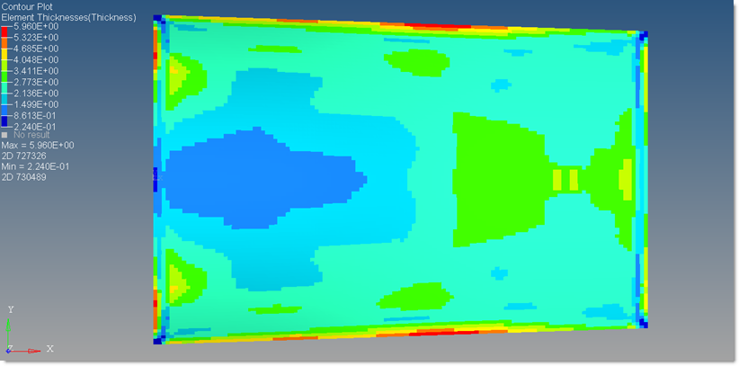
View the Element Thickness Results
-
From the OptiStruct panel, click HyperView.
HyperView launches and opens the fairing_freesize.mvw session file, which contains three pages with the results from three H3D files.
- Page 1
- Optimization results in fairing_freesize_des.h3d.
- Page 2
- Analysis results of subcase 1 in fairing_freesize_s1.h3d.
- Page 3
- Analysis results of subcase 2 in fairing_freesize_s2.h3d.
- Verify that you are on page 1.
-
On the Results toolbar, click
 to open the
Contour panel.
to open the
Contour panel.
-
In the Results Browser, select the last iteration.
Figure 4. Select the Final Iteration 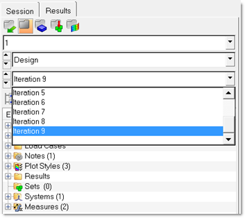
- Click Apply.
-
On the Standard Views toolbar, click
 to view the results in the X-Y plane.
View the Ply Thickness Results
- From the Contour panel, set the Result type to Ply Thicknesses (s).
-
Select the other plot options as indicated in Figure 6.
Figure 6. Ply Thicknesses Contour Plot 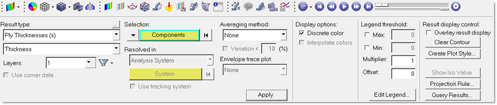
- In the Results Browser, select the last iteration.
-
Click Apply.
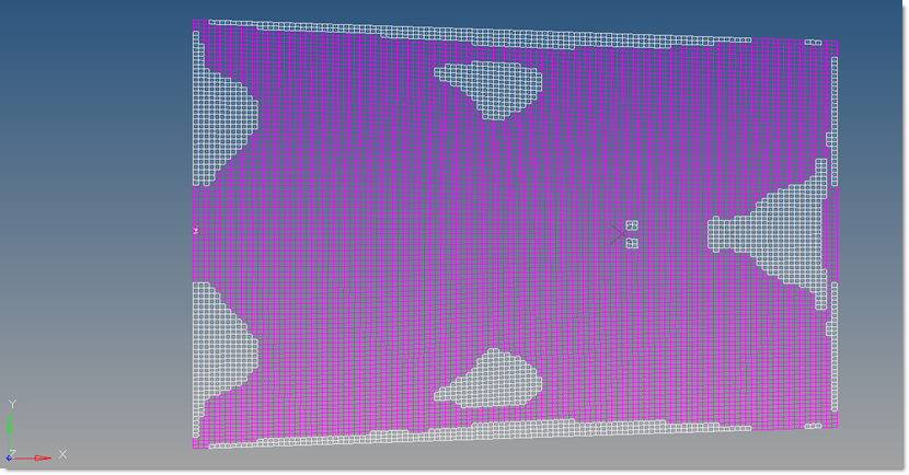
The thickness distribution of 0 degree super ply is generated. It represents the ply shapes and patch locations of the 0 degree ply bundles.
Figure 7. Ply Thickness Contour Plot . of the 0 degree super-ply 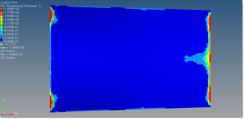
-
Create the ply thickness contours for super-ply 2 (45°), 3 (-45°), and 4 (90°)
by selecting Layers 2, 3 and 4, respectively in the Contour panel.
Due to the balance constraint applied, the thickness distribution of the +45° and the -45° super ply are the same.
Figure 8. Ply Thickness Contour Plot. of the -45/+45 degree super-plies 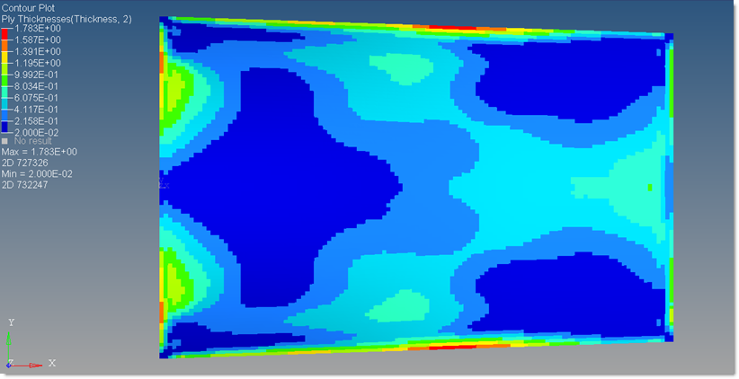
Figure 9. Ply Thickness Contour Plot . of the 90 degree super-ply 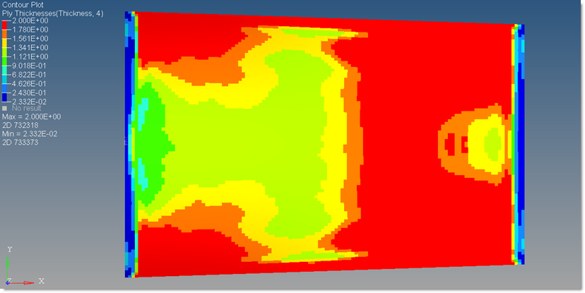
View the Ply Bundles through Element Sets
- Go back to the HyperMesh session.
- Import the solver deck fairing_freesize_sizing.*.inc, located in the same directory where the file fairing_freesize.fem, into the current session.
-
In the Model Browser, right-click on the Load
Collectors folder and select Hide from
the context menu.
The display of all load collectors is turned off.
- From the Analysis page, click the entity sets panel.
-
Click review and select set
5.
set 5 represents the ply bundle 1 of the +45° orientation super-ply.Tip: You can review ply bundles in the Model Browser, Plies folder. Click any ply to view it's corresponding card data in the Entity Editor.
Figure 10. Element set 5 representing ply bundle 1 of the +45 degree super ply 
-
Review the element sets 6 though 8.
Figure 11. Element set 6 representing ply bundle 2 of the +45 degree super ply 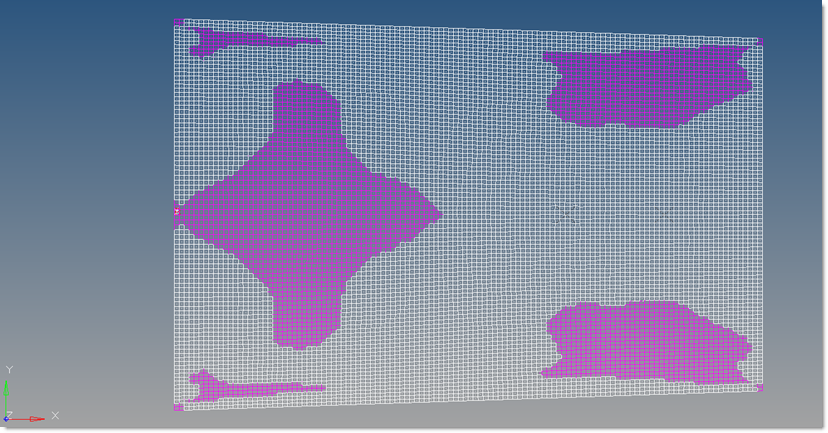
Figure 12. Element set 7 representing ply bundle 3 of the +45 degree super ply 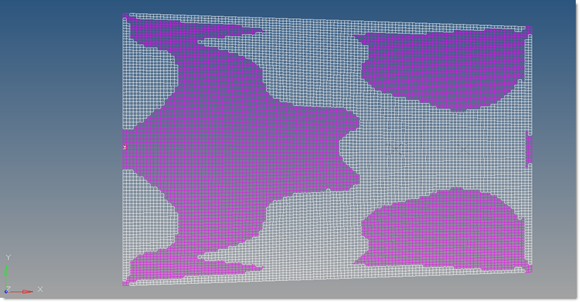
Figure 13. Element set 8 representing ply bundle 4 of the +45 degree super ply